.webp)
Free MLOps Course for Data Scientists: Day 3 - Machine Learning Pipelines
A practical guide to ML pipelines for Data Scientists: preprocessing, feature engineering, training, and inference pipelines explained with Python code examples and implementation best practices.

Welcome to Day 3 of my 5-day MLOps Course for Data Scientists.
Day 1 - Production ML System Components
Day 2 - Databases and Data Processing
When you want to deploy a model to production, you quickly realize that the model itself is only a small part of the system. You see that there is data that needs to be processed, features that need to be computed, predictions that need to be delivered, and all of this has to happen automatically and reliably.
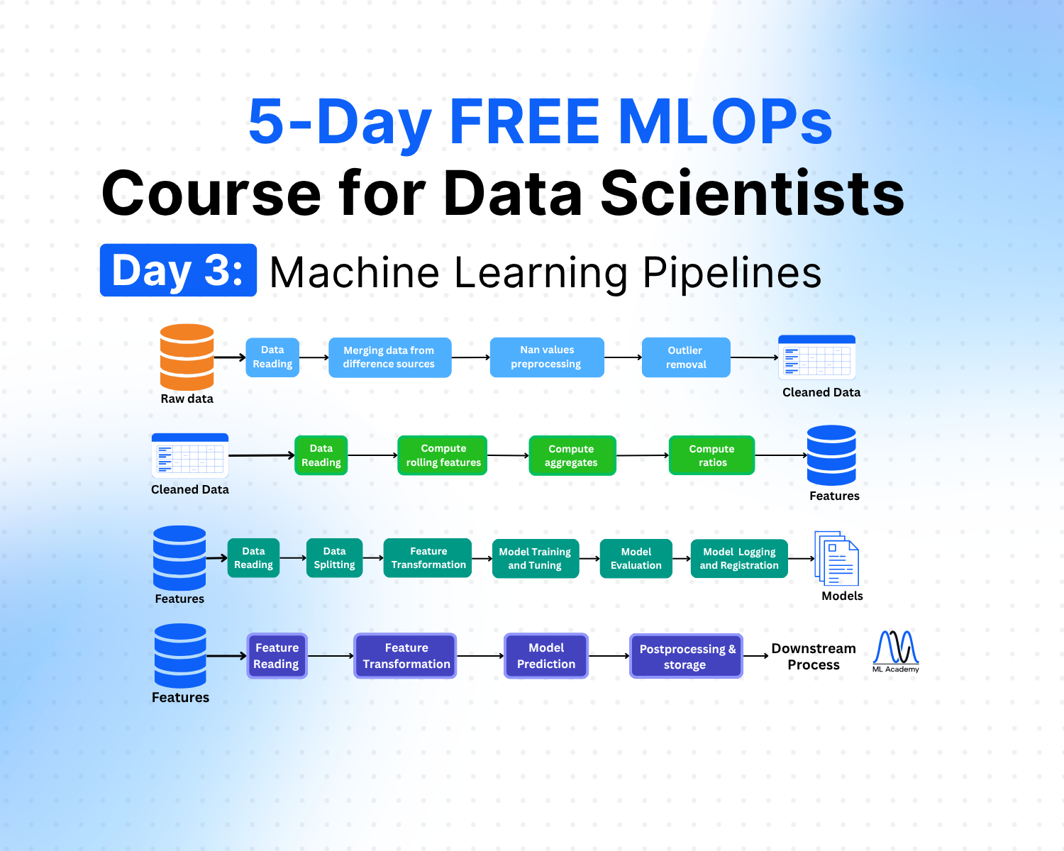
These data transformations and model operations happen in ML pipelines. This lesson covers three pipeline types that sit at the core of most ML solutions: Preprocessing and Feature Engineering Pipelines, Training Pipeline, and Inference Pipeline.
Each pipeline has a distinct responsibility. The preprocessing and feature engineering pipelines turn raw data into model-ready features. The training pipeline takes those features and produces a trained, evaluated, and registered model. The inference pipeline delivers predictions from that model on a schedule or on demand.
Together, these components form the operational backbone of any ML solution, as we can see in the figure below.
1. What is an ML Pipeline?
An ML pipeline is a structured sequence of steps (nodes) that takes data from raw input through processing, model training, evaluation, and deployment in a repeatable, automated way.
ML Pipelines are usually represented by Directed Acyclic Graphs (DAGs).
A DAG is a sequence of steps (operations) where each step runs only after its dependencies are completed, and the steps never form loops.
Here’s a simple example of an ML Pipeline represented as a DAG.
%20(1).png)
In this simple example, the pipeline integrates the steps from raw data up to model training. However, in reality, we divide such pipelines into several pipelines, where each pipeline does a certain task.
In the vast majority of cases, we have 3 types of ML pipelines:
- Feature Engineering
- Training
- Inference
Such a pipeline combination is often referred to as FTI (Feature, Training, Inference) and is commonly used in books and other materials.
However, I also like to separate a Preprocessing Pipeline that comes before Feature Engineering pipelines. This is because often in real-world messy data, we have to perform quite a few steps to prepare the data before we actually do feature engineering.
In this course, I will describe it separately, but describe it together with the Feature Engineering pipeline to follow the FTI convention.
2. Preprocessing & Feature Engineering Pipelines
A Preprocessing Pipeline is the one where raw data is transformed into a clean and consistent format before it can be used in feature engineering. Without preprocessing, models risk learning from noise, inconsistencies, or irrelevant signals.
Task Examples:
- Handling missing values, outliers, and duplicates
- Merging data from different sources
- Encoding categorical variables
Here’s an example overview of a Preprocessing ML Pipeline.
%20(2).png)
Here’s a simple example of what such a Preprocessing Pipeline might look like in code.
import pandas as pd
from pathlib import Path

config = {
    "file_paths": ["sensors.csv", "labels.parquet"],
    "merge_on": "timestamp",
    "merge_how": "outer",
    "nan_strategy": "median",      # "mean" | "median"
    "iqr_multiplier": 1.5,         # IQR fence width
    "outlier_quantiles": [0.25, 0.75],
}


class PreprocessingPipeline:
    """End-to-end preprocessing: read → merge → impute → remove outliers."""

    def __init__(self, config: dict):
        self.cfg = config
        self.df = None

    def read_data(self):
        """Load each file into a DataFrame based on its extension."""
        readers = {".csv": pd.read_csv, ".parquet": pd.read_parquet, ".xlsx": pd.read_excel}
        self._frames = [readers[Path(p).suffix](p) for p in self.cfg["file_paths"]]
        return self

    def merge_sources(self):
        """Merge all loaded DataFrames into one."""
        self.df = self._frames[0]
        for f in self._frames[1:]:
            self.df = self.df.merge(f, on=self.cfg["merge_on"], how=self.cfg["merge_how"])
        return self

    def preprocess_nan(self):
        """Fill numeric NaNs using the configured strategy (mean or median)."""
        num = self.df.select_dtypes(include="number").columns
        fill = {"mean": self.df[num].mean(), "median": self.df[num].median()}
        self.df[num] = self.df[num].fillna(fill[self.cfg["nan_strategy"]])
        return self

    def remove_outliers(self):
        """Drop rows where any numeric column falls outside IQR bounds."""
        num = self.df.select_dtypes(include="number").columns
        mask = pd.Series(True, index=self.df.index)
        k = self.cfg["iqr_multiplier"]
        for col in num:
            q1, q3 = self.df[col].quantile(self.cfg["outlier_quantiles"])
            mask &= self.df[col].between(q1 - k*(q3-q1), q3 + k*(q3-q1))
        self.df = self.df[mask]
        return self

    def run(self) -> pd.DataFrame:
        """Execute the full pipeline and return cleaned DataFrame."""
        self.read_data()
        self.merge_sources()
        self.preprocess_nan()
        self.remove_outliers()
        return self.df

# Usage
cleaned_df = PreprocessingPipeline(config).run()
A Feature Engineering Pipeline is responsible for creating features that are then used by a Machine Learning model
Task Examples:
- Deriving new features (e.g., ratios, rolling averages, time lags)
- Extracting domain-specific attributes (e.g., distance between GPS coordinates)
- Representing complex data (e.g., embeddings for text, image augmentation for vision tasks)
%20(1).png)
Here’s a simple example of what such a Preprocessing Pipeline might look like in code.
import pandas as pd
from pathlib import Path


config = {
    "file_path": "cleaned_data.csv",
    "sort_by": "timestamp",
    "rolling_window": 3,           # rolling window size
    "rolling_cols": ["sensor_1", "sensor_2"],
    "agg_cols": ["sensor_1", "sensor_2"],
    "agg_funcs": ["mean", "std", "min", "max"],
    "ratio_pairs": [               # (numerator, denominator)
        ("sensor_1", "sensor_2"),
    ],
}


class FeatureEngineeringPipeline:
    """Feature engineering: read → rolling features → aggregates → ratios."""

    def __init__(self, config: dict):
        self.cfg = config
        self.df = None

    def read_data(self):
        """Load cleaned data from disk based on file extension."""
        readers = {".csv": pd.read_csv, ".parquet": pd.read_parquet, ".xlsx": pd.read_excel}
        self.df = readers[Path(self.cfg["file_path"]).suffix](self.cfg["file_path"])
        if self.cfg.get("sort_by"):
            self.df = self.df.sort_values(self.cfg["sort_by"]).reset_index(drop=True)
        return self

    def compute_rolling_features(self):
        """Add rolling mean and std columns for configured columns and window size."""
        w = self.cfg["rolling_window"]
        for col in self.cfg["rolling_cols"]:
            self.df[f"{col}_roll_mean_{w}"] = self.df[col].rolling(w).mean()
            self.df[f"{col}_roll_std_{w}"]  = self.df[col].rolling(w).std()
        return self

    def compute_aggregates(self):
        """Add global aggregate features (mean, std, min, max) per configured column."""
        for col in self.cfg["agg_cols"]:
            for fn in self.cfg["agg_funcs"]:
                self.df[f"{col}_agg_{fn}"] = self.df[col].transform(fn)
        return self

    def compute_ratios(self):
        """Add ratio features for each configured (numerator, denominator) pair."""
        for num, den in self.cfg["ratio_pairs"]:
            self.df[f"ratio_{num}_to_{den}"] = self.df[num] / self.df[den].replace(0, float("nan"))
        return self

    def run(self) -> pd.DataFrame:
        """Execute the full pipeline and return the feature DataFrame."""
        self.read_data()
        self.compute_rolling_features()
        self.compute_aggregates()
        self.compute_ratios()
        return self.df


# Usage
features = FeatureEngineeringPipeline(config).run()
3. Training ML Pipeline
The Training Pipeline is the automated sequence that takes data and produces a trained, evaluated, and registered model.
The word that matters in the definition is automated. A notebook is a sequence of cells you ran in some order, with a state that exists only in your kernel. A training pipeline is code that runs the same way every time, on demand or on a schedule, with no human in the loop.
What a training pipeline actually does
A typical training pipeline executes several main steps shown in the figure below.
%20(1).png)
Let’s break each step down.
1. Data Reading/Ingestion
In this step, the pipeline gets the data from either an offline feature store or right from the Feature Engineering pipeline.
2. Data Splitting
Here, the pipeline separates data into train, validation, and test sets.
The splitting can be different depending on the problem type. For instance, for time-series problems, this must be time-based. For classification with a minority class, class stratification must be considered.
3. Feature Transformation
Here, we fit transformations like scaling on the training set only, then apply them to the validation and test sets.
We also need to save the fitted artifacts because the inference pipeline will need exactly the same transformations.
4. Model Training & Hyperparameter Tuning
Finally, we run the actual model fitting. Often, we need to tune model hyperparameters (e.g., number of neural network layers, learning rate, tree depths, etc.), for which various methods can be used, for example, Bayesian Optimization.
5. Model Evaluation
Here, we compute metrics on the test set, e.g.m, accuracy, F1, AUC, RMSE.
6. Logging and registration
Finally, we write parameters, metrics, the model file, and the preprocessing artifacts to the experiment tracking system and the Model Registry.
Here's a code example of such a Training ML Pipeline.
import pandas as pd
from pathlib import Path
from sklearn.model_selection import train_test_split, GridSearchCV
from sklearn.preprocessing import StandardScaler, MinMaxScaler
from sklearn.ensemble import RandomForestClassifier
from sklearn.metrics import classification_report
from xgboost import XGBClassifier
import mlflow, mlflow.sklearn


config = {
    "file_path": "features.parquet",
    "target_col": "fault_flag",
    "test_size": 0.2,
    "random_state": 42,
    "scaler": "standard",           # "standard" | "minmax"
    "model": "random_forest",       # "random_forest" | "xgboost"
    "param_grid": {"n_estimators": [100, 200], "max_depth": [3, 5]},
    "cv_folds": 3,
    "mlflow_experiment": "training_pipeline",
    "mlflow_model_name": "fault_classifier",
}

class TrainingPipeline:
    """Training pipeline: read → split → transform → train/tune → evaluate → log."""

    def __init__(self, config: dict):
        self.cfg = config
        self.df = None
        self.X_train = self.X_test = self.y_train = self.y_test = None
        self.model, self.best_params, self.metrics = None, {}, {}

    def read_data(self):
        """Load feature data from disk based on file extension."""
        readers = {".csv": pd.read_csv, ".parquet": pd.read_parquet, ".xlsx": pd.read_excel}
        self.df = readers[Path(self.cfg["file_path"]).suffix](self.cfg["file_path"])
        return self

    def split_data(self):
        """Split DataFrame into train/test sets."""
        X = self.df.drop(columns=[self.cfg["target_col"]])
        y = self.df[self.cfg["target_col"]]
        self.X_train, self.X_test, self.y_train, self.y_test = train_test_split(
            X, y, test_size=self.cfg["test_size"], random_state=self.cfg["random_state"]
        )
        return self

    def transform_features(self):
        """Scale numeric features using the configured scaler."""
        scaler = {"standard": StandardScaler(), "minmax": MinMaxScaler()}[self.cfg["scaler"]]
        self.X_train = scaler.fit_transform(self.X_train)
        self.X_test  = scaler.transform(self.X_test)
        return self

    def train_and_tune(self):
        """Train model with GridSearchCV over the configured param grid."""
        base = {"random_forest": RandomForestClassifier, "xgboost": XGBClassifier}[self.cfg["model"]]
        search = GridSearchCV(base(random_state=self.cfg["random_state"]), self.cfg["param_grid"], cv=self.cfg["cv_folds"])
        search.fit(self.X_train, self.y_train)
        self.model, self.best_params = search.best_estimator_, search.best_params_
        return self

    def evaluate(self):
        """Evaluate model on test set and store metrics."""
        report = classification_report(self.y_test, self.model.predict(self.X_test), output_dict=True)
        self.metrics = {k: report["weighted avg"][k] for k in ["precision", "recall", "f1-score"]}
        self.metrics["accuracy"] = report["accuracy"]
        return self

    def log_and_register(self):
        """Log params, metrics, and model to MLflow and register."""
        mlflow.set_experiment(self.cfg["mlflow_experiment"])
        with mlflow.start_run():
            mlflow.log_params(self.best_params)
            mlflow.log_metrics(self.metrics)
            mlflow.sklearn.log_model(self.model, "model", registered_model_name=self.cfg["mlflow_model_name"])
        return self

    def run(self) -> dict:
        """Execute the full training pipeline and return evaluation metrics."""
        self.read_data()
        self.split_data()
        self.transform_features()
        self.train_and_tune()
        self.evaluate()
        self.log_and_register()
        return self.metrics
# Usage
metrics = TrainingPipeline(config).run()
When it runs
There are many different scenarios when we can trigger Training Pipelines. These are the most common ones.
- On-demand — you decided that you need to re-train the model for whatever reason.
- Scheduled — for example, weekly or monthly retraining (most common default)
- Performance-based — model error crosses a threshold, retraining fires automatically
- Drift-based — input distributions have shifted enough that the current model is suspect
4. Inference Pipeline
The Inference Pipeline is the path data takes from new inputs, through feature transformation and the trained model, to a delivered prediction.
Inference comes in two main forms with different architectures that are related to the Data Processing part discussed above.
Batch Inference
Batch Inference runs predictions on the batch dataset on a schedule. For example, a daily churn classification job: every night the pipeline scores all active customers as churn / non-churn, writes the results to a database (customer_id, churn_score, scored_at, model_version)
Real-Time Inference
Real-Time Inference serves predictions instantly via an API, usually within tens of milliseconds. It is used when the prediction has to influence something happening right now, for example, ranking videos as a user opens the app or approving a transaction.
Regardless of flavor, the steps of the pipeline are usually similar to the one shown in the figure below.
%20(2).png)
Let’s break it down.
1. Feature Reading
Here, there are usually two ways of doing this:
Take features from Online Store — features that were already computed and stored ahead of time (e.g., the user's 7-day average watch time, updated continuously in the background).
Take them straight from the Feature Engineering Pipeline — the incoming data is run through the same feature engineering pipeline used in training, and the resulting features are consumed directly, without being stored first.
2. Feature Transformation
Before the model can use the features, they have to be put into the exact same form they had during training, meaning the same scaling, encoding, and imputation.
We have to reuse the transformations that were fitted during training and saved as artifacts. Don't fit new ones here.
3. Prediction
Here, we load the trained model from the Model Registry and run it on the prepared features from a Feature Store or from a Feature Engineering Pipeline.
Depending on the inference type, two different strategies are usually used:
- Batch Inference: the pipeline loads the model once at the start of the run and calls .predict() on the provided batch.
- Real-time Inference: the model runs behind a serving API (FastAPI, BentoML, KServe). Each incoming request triggers an API call that runs the prepared features through the model and returns a single prediction within the target latency
In both cases, load the model by its registered alias or by the registry stage, not by a file path.
Instead of pointing at a specific version number, inference asks the registry for the model behind an alias like @champion or @production or from the Production model registry stage and the registry resolves it to whichever version is currently assigned.
4. Postprocessing & storage
In many cases, the model's raw output is transformed into some business-related output. It applies whatever logic sits between the model's raw score and the decision, for example:
- Thresholds — convert a probability into a decision (e.g., churn_score > 0.7 → flag the customer for a retention campaign).
- Business rules — override or constrain predictions (e.g., never recommend a video the user has already watched, never flag a whitelisted account).
- Ranking logic — sort and trim outputs (e.g., take the top 10 videos out of thousands of scored candidates).
Then the result is stored or returned, depending on the inference type:
- Batch: write the predictions to a database
- Real-time: return the predictions directly in the API response, often caching them first, for example, in Redis, and only then are they stored in a database if required.
Here's what such an Inference Pipeline might look like in code.
import pandas as pd
from pathlib import Path
from sklearn.preprocessing import StandardScaler, MinMaxScaler
import mlflow.sklearn


config = {
    "file_path": "features.parquet",
    "model_uri": "models:/fault_classifier/Production",
    "scaler": "standard",           # "standard" | "minmax"
    "proba_threshold": 0.5,
    "output_path": "predictions.parquet",
}


class InferencePipeline:
    """Inference pipeline: read → transform → predict → postprocess & store."""

    def __init__(self, config: dict):
        self.cfg = config
        self.df = None
        self.X = None
        self.predictions = None

    def read_features(self):
        """Load feature data from disk based on file extension."""
        readers = {".csv": pd.read_csv, ".parquet": pd.read_parquet, ".xlsx": pd.read_excel}
        self.df = readers[Path(self.cfg["file_path"]).suffix](self.cfg["file_path"])
        self.X = self.df.copy()
        return self

    def transform_features(self):
        """Scale numeric features using the configured scaler."""
        scaler = {"standard": StandardScaler(), "minmax": MinMaxScaler()}[self.cfg["scaler"]]
        self.X = scaler.fit_transform(self.X)
        return self

    def predict(self):
        """Load model from MLflow registry and run predictions."""
        model = mlflow.sklearn.load_model(self.cfg["model_uri"])
        proba = model.predict_proba(self.X)[:, 1]
        self.predictions = (proba >= self.cfg["proba_threshold"]).astype(int)
        self.df["prediction"] = self.predictions
        self.df["proba"] = proba
        return self

    def postprocess_and_store(self):
        """Add metadata and write predictions to output path."""
        self.df["predicted_at"] = pd.Timestamp.utcnow()
        self.df.to_parquet(self.cfg["output_path"], index=False)
        return self

    def run(self) -> pd.DataFrame:
        """Execute the full inference pipeline and return predictions DataFrame."""
        self.read_features()
        self.transform_features()
        self.predict()
        self.postprocess_and_store()
        return self.df


# Usage
results = InferencePipeline(config).run()
5. ML Pipeline Frameworks
There are many frameworks you can use to build and orchestrate ML pipelines. Before picking one, it helps to understand an important distinction: some tools are ML pipeline frameworks, and some are orchestrators. They are not the same thing.
An ML pipeline framework, like Kedro, is focused on creating reproducible, modular, and maintainable pipeline code.
An orchestration framework, like Prefect or Airflow, is focused on scheduling, monitoring, and managing pipeline execution.
In practice, you can use both together — Kedro to structure the pipeline code, and Prefect to run and monitor it in production.
Here are the most commonly used tools:
Kedro is an open-source Python framework for creating reproducible and modular ML pipelines. It enforces clean code structure, standardizes the project layout, and integrates well with other tools. It also comes with Kedro-viz, a pipeline visualization tool that makes it easy to inspect and debug your DAGs. Good choice if you want to write well-structured pipeline code.
Prefect is an orchestration framework built around Python functions and decorators. It feels like normal code, has a low learning curve, and is easy to set up locally and deploy to the cloud. Tasks can be scheduled, retried, and skipped. Good choice as a first orchestration tool or for production ML pipelines.
Airflow is a widely used orchestration platform built around DAG objects and operators. It is the standard in large-scale data platforms and enterprise data teams. The learning curve is steeper, and the local setup requires a scheduler, database, and workers. Good choice if you are joining a team that already uses it.
Metaflow is developed by Netflix and is designed specifically for data scientists. It handles data versioning, compute scaling, and deployment with minimal configuration. Good choice for teams that want to move fast without managing infrastructure.
ZenML is a framework that sits on top of your existing tools and standardizes the pipeline interface across different backends. It lets you switch between local execution and cloud deployment without changing your pipeline code. Good choice if you want flexibility across environments.
Here’s the summary
%20(2).png)
6. ML Pipeline Implementation - best practices
1. Use a Class
Wrap your pipeline in a class. Without a class, you end up with loose functions, scattered variables, and no clear structure. A class keeps everything in one place and makes the pipeline reusable. The example of how to do that you can see in the figures above.
2. Use Config
Never hardcode parameters inside methods. If a value changes, for instance, you get a new threshold, a column name, a file path, you change it only in one place - your config file. Again, you can see the examples above.
3. One Class Method, One Responsibility
Each method should do exactly one thing. If a method cleans data and also computes features, split it. One responsibility per method makes the pipeline easier to test, debug, and extend.
Here's the example.
# wrong — two responsibilities in one method
def clean_and_engineer(self, df):
    df = df.fillna(df.median())
    df["amount_ratio"] = df["amount"] / df["total"]
    return df


# right — each method has one job
def fill_missing_values(self, df):
    return df.fillna(df.median())

def compute_ratios(self, df):
    df["amount_ratio"] = df["amount"] / df["total"]
    return df
4. Use a run Method
The run method is the only method an external caller should ever need. It defines the order of execution and passes data between steps. Again, we did exactly that in the pipeline examples above
5. Save Artifacts
Any transformation fitted during preprocessing, feature engineering, and training, e.g., a scaler, must be saved. The inference pipeline will need to apply the exact same transformation to new data.
If you refit on new data, the parameters will be different, and your model will see data it was never trained on.
Summary
An ML pipeline is a structured, automated sequence of steps that takes raw data all the way to a delivered prediction. Most ML systems are built around three core pipeline types which is often called FTI:
1. Preprocessing Pipeline:
Cleans raw data: merges sources, handles NaNs, removes outliers. Runs upstream of training, either on a schedule or triggered when new raw data arrives.
2. Feature Engineering Pipeline:
Creates model-ready features: rolling stats, aggregates, ratios. Runs after preprocessing, on a schedule or on demand, feeding either a Feature Store or directly into training.
3. Training Pipeline:
Produces a trained model: splits data, scales features, tunes hyperparameters, evaluates, and logs everything to MLflow. Runs on-demand, on a schedule (e.g. weekly/monthly), when model performance drops below a threshold, or when input distributions drift.
4. Inference Pipeline
Delivers predictions: reads features, applies the same transformations as training, runs the model, postprocesses results, and stores or returns them. Runs on a schedule (batch) or in real-time per request (API).
Implementation Best Practices
- Use a class — keeps the pipeline structured and reusable
- Use a config dict — all parameters in one place, never hardcoded
- One method, one responsibility — easier to test, debug, and extend
- Use a run() method — single entry point that defines execution order
- Save artifacts — scalers and encoders fitted during training must be reused at inference, not refitted
In the next lesson, we will cover Feature Store, Experiment Tracking and Model Registry.
Related Articles


Free MLOps Course for Data Scientists: Day 2 - Databases and Data Processing
A five-part guide to data storage and processing for production ML systems: relational, column-oriented, vector, and key-value databases, plus streaming and batch processing explained for Data Scientists.
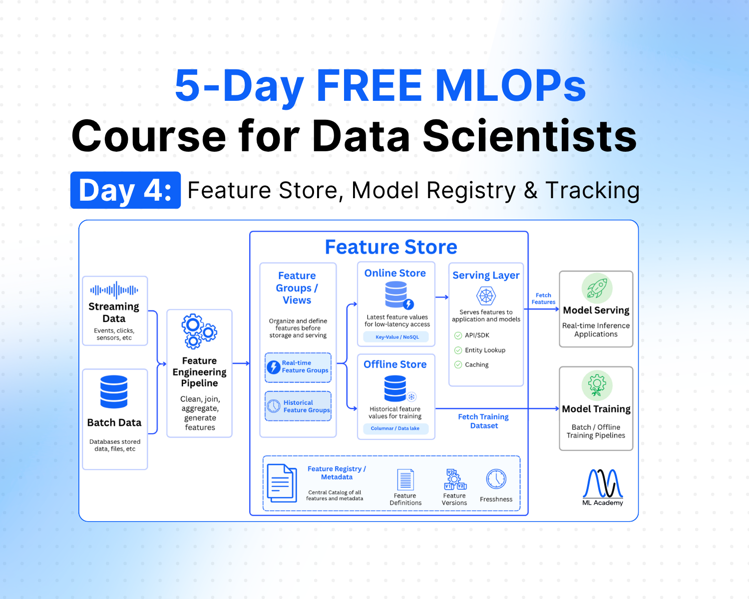
Free MLOps Course for Data Scientists: Day 4 - Feature Store, Model Registry and Experiment Tracking
A practical guide to feature stores, experiment tracking, and model registry for Data Scientists: what each component does, when to use them, and how they connect in a production ML system.
Ready to transform your ML career?
Join ML Academy and access free ML Courses, weekly hands-on guides & ML Community