.webp)
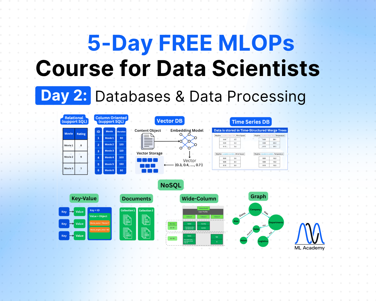
Free MLOps Course for Data Scientists: Day 2 - Databases and Data Processing
A five-part guide to data storage and processing for production ML systems: relational, column-oriented, vector, and key-value databases, plus streaming and batch processing explained for Data Scientists.

Welcome to Day 2 of my 5-day MLOps Course for Data Scientists.
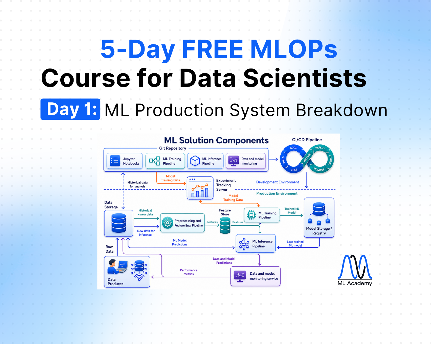
Day 1 - Production ML System Components
Today, we will learn about two foundational layers of ML systems.
The first layer is data storage. This is where all your data sits, and the choice of storage technology directly impacts how fast your system can retrieve it.
The second layer is data processing, which is how raw data gets transformed into something a model can actually use.
Now, as a Data Scientist, you can get far without knowing either. Often, we just use Pandas to read a CSV, train a model, and go to get a coffee.
But the moment your work moves into production, these two layers become unavoidable. The storage technology determines whether your feature pipeline runs in seconds or hours, and the processing architecture determines whether your model scores a transaction in 50 milliseconds or waits until the next morning batch job.
So today, we will cover both. What the main storage types are and when to use them, and how streaming and batch processing differ in practice.
1. Data Storage
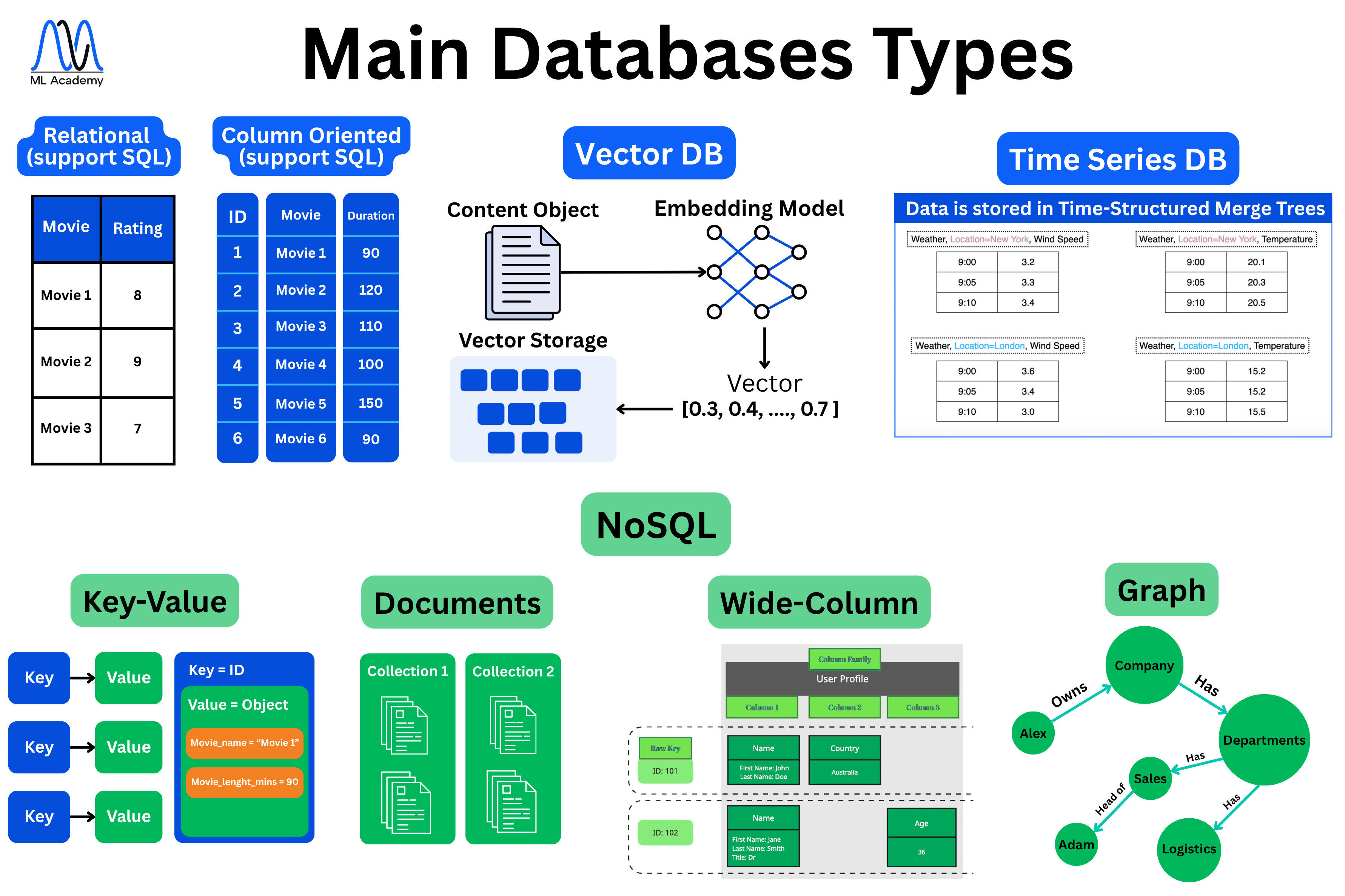
This is the place where everything starts. No ML solution can be built without data. The choice of storage technology significantly impacts both the speed of your ML system and its maintainability over time. Here’s an overview of the main database types in production ML systems.
This is the place where everything starts. No ML solution can be built without data. The choice of storage technology significantly impacts both the speed of your ML system and its maintainability over time. Here’s an overview of the main database types in production ML systems.
Now, let’s break down some of the most important and commonly used DB types in Production ML systems.
Relational (SQL)
Relational databases are the oldest and most battle-tested way to store structured data. The core idea is simple: data lives in tables with rows and columns, where each table represents one entity — users, orders, products.
The most common engines you'll run into are MySQL, PostgreSQL, SQLite, and Microsoft SQL Server. They each have their own tradeoffs, but all of them speak the same core language: SQL.
%20(1).png)
What makes relational databases attractive is how much you get out of the box. ACID transactions ensure your data stays consistent even when something fails mid-operation. ACID stands for Atomicity, Consistency, Isolation, and Durability.
Atomicity means a transaction is all or nothing. This means that if a multi-step operation fails halfway through, the whole thing rolls back.
Consistency means the database enforces your rules at all times. If you have a constraint that an order must always reference a valid customer, the database will reject any transaction that tries to create an order without one. You can never end up with data that violates your schema rules, regardless of what went wrong during the transaction.
Isolation means concurrent transactions don't interfere with each other.
Durability means once a transaction commits, it is permanently saved. The way this works is that the database writes every transaction to a log on disk before confirming success. This log is called a Write-Ahead Log, or WAL. So even if the server crashes the next second, when it restarts, it replays that log and recovers any committed transactions. You never lose a confirmed write.
Together, these four properties are what make relational databases trustworthy for anything where partial writes or data corruption are not acceptable.
Beyond transactions, SQL itself is expressive enough to handle joins, filters, aggregations, and constraints without any additional tooling. On top of that, you have decades of community support, mature indexing strategies, and operational tooling that's been refined over the years.
Column-Oriented
Column-oriented databases store data by column rather than by row. In a row-oriented database, all fields for a single record are stored together on disk. In a column-oriented database, all values for a single column are stored together. So instead of storing "user 1's entire record, then user 2's entire record," you store "all user IDs, then all user names, then all signup dates."
%20(1).png)
This makes a significant difference for analytical workloads. When you run a query like "give me the average order value across 10 million rows," a column-oriented database only reads the order value column. A row-oriented database reads every row in full, including all the fields you don't need. The result is dramatically less I/O and much faster aggregations on large datasets.
The tradeoff is that column-oriented databases are poor at row-level operations. Inserting or updating a single record means touching many separate column files on disk, which is expensive. This is why they are not suited for transactional workloads where you frequently write or update individual records. They are also less efficient when you regularly need to retrieve full rows, since reconstructing a complete record requires reading across many column files.
The most common engines you'll run into are ClickHouse, DuckDB, Apache Druid, Snowflake, Amazon Redshift, and Google BigQuery. They each have their own tradeoffs around latency, scale, and cost, but all of them are optimized for the same core use case: fast analytical queries on large datasets.
Where they shine is business intelligence, data warehousing, log and event analytics, and any workload that involves scanning and aggregating large volumes of structured data. If your queries are more "compute this metric across all rows" than "fetch this specific record," a column-oriented database is almost always the right choice.
Vector DB
Vector databases are purpose-built for one thing: storing and searching embeddings. An embedding is a numerical representation of a piece of content — a document, an image, an audio clip — produced by a machine learning model. That representation is a vector, which is just a list of numbers like [0.30, 0.40, ..., 0.70].
The key insight is that similar content produces similar vectors, so finding related items becomes a mathematical problem of finding vectors that are close to each other in high-dimensional space.
%20(1).png)
The workflow is quite simple. You take a content object, pass it through an embedding model, get a vector back, and store that vector in the database. At query time, you do the same thing to your query, i.e., convert it to a vector and then ask the database to find the most similar vectors it has stored. This is called nearest-neighbor search, and it is what vector databases are specifically optimized for.
What makes them attractive is speed at scale. Traditional databases can't efficiently answer "find me the 10 most similar items to this query" across millions of records. Vector databases use specialized index structures like HNSW or IVF to make that search fast, even at large collections. They also work across data types, like text, images, and audio, as long as you have an embedding model that can encode them.
But as always, there are tradeoffs. Search quality depends entirely on the quality of your embeddings. If your embedding model doesn't capture the right semantics, your search results will be poor regardless of how well-tuned the database is. The search itself is also approximate by default, meaning it trades some accuracy for speed.
The most common engines you'll run into are Pinecone, Milvus, Weaviate, Qdrant, Chroma, and Vespa. Each has different tradeoffs around hosting, scale, and filtering capabilities, but all of them are built around the same core operation: fast similarity search over high-dimensional vectors.
Where Vector DBs work best is anywhere you need semantic retrieval. For instance, it’s RAG pipelines for LLMs, semantic search over documents, recommendation systems, image search, and anomaly detection.
Essentially, it’s any problem where "find me things similar to this" is the core query pattern. If your application relies on embeddings, a vector database is almost always the right storage layer.
Key-Value
Key-value databases are the simplest storage model you'll encounter. The entire data model is exactly what the name says: you store a value under a key, and you retrieve it by that key. There are no tables, no schemas, no joins. You put something in, you get something out. But here, this simplicity is the main point.
The way this works in practice is that the database maintains an in-memory hash map where each key maps directly to its value. Because there is no query parsing, no index traversal, and no disk seek involved, lookups are extremely fast, typically sub-millisecond. This is why Redis, the most widely used key-value store, is almost always the first choice when an application needs a caching layer.
.png)
The value itself can be almost anything. In Redis specifically, values can be strings, lists, sets, sorted sets, hashes, or even more specialized structures like streams and bitmaps.
This flexibility means Redis is used for far more than simple caching. It can be used for session storage, rate limiting, leaderboards, pub/sub messaging, and real-time counters.
However, key-value databases are only efficient when you know the exact key you're looking for. There is no way to query by value, filter across records, or express relationships between keys.
For instance, if you need to ask, "give me all users who signed up last week," a key-value store has no good answer. You'd need a different database for that. Memory cost is also a consideration because storing everything in RAM is fast but expensive, so key-value stores are typically used for hot data rather than as a primary store for large datasets.
2. Data Processing (Streaming / Batch)
Now, let's talk about data processing. This part of ML Solutions is responsible for processing the data and directing it to the right process.
There are 2 main types of data processing in ML applications - streaming and batch. Below you can see a schematic representation of these different approaches with a detailed description later on.
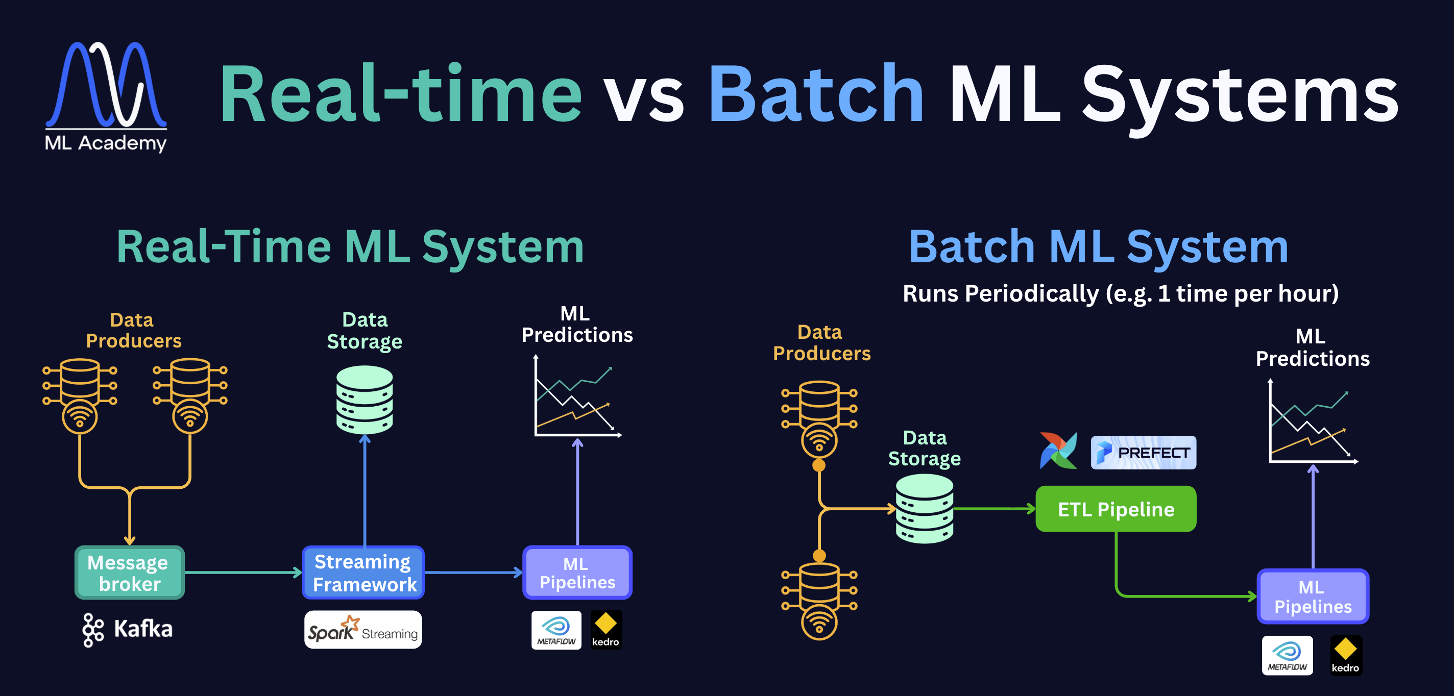
On the left is a Real-Time ML System. Data producers, like sensors, apps, or services, send data into a message broker (Kafka), which acts as a buffer. A streaming framework like Spark Streaming picks it up immediately and passes it to the ML pipelines. The whole process happens within milliseconds.
On the right is a Batch ML System. Data from multiple producers lands in storage first. On a schedule, for example, once an hour, an ETL pipeline wakes up, pulls that accumulated data, transforms it, and hands it off to the ML pipelines. Nothing happens in between runs; the system simply waits for the next trigger.
The choice between the system types is driven entirely by how quickly the business needs results. For instance, in many demand forecasting systems, the training pipeline runs on a schedule and can afford to wait for a full batch of sales data to accumulate.
In a fraud detection system, the model has to evaluate a transaction before it completes, which means latency is measured in milliseconds, not hours.
Common tools for streaming include message brokers like Apache Kafka or Amazon Kinesis to move data, and stream processors like Apache Flink or Kafka Streams to transform it.
For batch, you'll typically see orchestrators like Apache Airflow or Prefect scheduling jobs, with Apache Spark handling the heavy distributed processing.
Let’s break each system down.
Streaming Data Processing
In the case of streaming, data is processed and served within milliseconds.
A typical example of it is fraud detection systems, where the ML system must identify if the transaction is fraudulent or not and prevent catastrophic consequences.
The tools that are typically used for these:
Message Brokers: Apache Kafka, Amazon Kinesis
Stream Processing: Apache Flink, Kafka Streams, Spark Streaming
Let’s break down the difference between Message Brokers and Stream Processing tools.
Kafka Message Broker
Here’s how message brokers work based on the Kafka example:
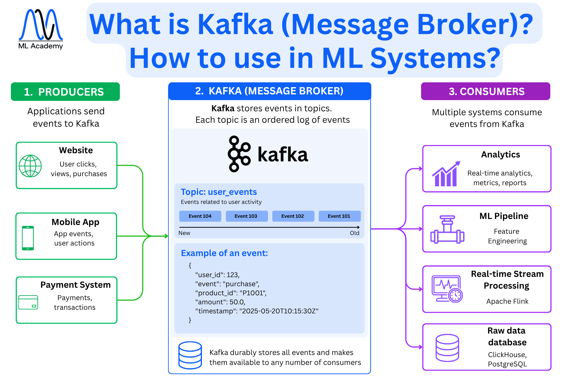
Kafka has three main roles: producers, a broker, and consumers.
Producers are the applications that send events into Kafka. In a typical ML system, these might be a website tracking user clicks and purchases, a mobile app sending user actions, or a payment system emitting transaction records.
The broker is Kafka itself. It receives events from producers and stores them in topics. A topic is an ordered, append-only log. In this log, events are written at one end and consumers read from any point in the log.
In the diagram, the topic is user_events, which holds events related to user activity. Each event is a structured record: a user_id, an event type like purchase, a product_id, an amount, and a timestamp. Kafka stores all events on disk and makes them available to any number of consumers independently. This means that one consumer's reading doesn't remove or block the event for another.
Consumers are the downstream systems that subscribe to a topic and process events as they arrive. From the same user_events topic, an analytics system might be computing real-time metrics, an ML pipeline doing feature engineering, and a monitoring system tracking observability metrics. The trick is that all are reading the same stream simultaneously.
This decoupling is what makes Kafka central to real-time ML systems. The producer doesn't need to know who will consume the data or when. You can add a new consumer, for example, a streaming processing tool, without touching any upstream code.
Apache Flink Streaming Processor
A message broker like Kafka moves events reliably from producers to consumers. It doesn't transform them. That's where a stream processing framework comes in.
Apache Flink reads from a Kafka topic and runs a processing pipeline on each event as it arrives. The pipeline has four steps: read the stream topic, filter events, transform data, and generate output. In the fraud detection example, this happens within milliseconds of the transaction hitting Kafka
This is how Streaming Processors work based on the Apache Flink example:
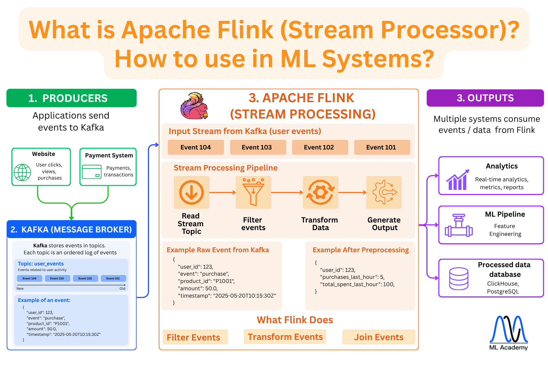
In this example, Flink computes aggregates over a time window, like how many purchases this user made in the last hour, and how much they spent. That's the feature your ML model actually needs to score fraud risk.
In many cases, the raw event might not be useful to the model directly, but the Flink-processed output can.
In the example pipeline above, Flink does three things:
Filter events — drop irrelevant events before they reach downstream systems.
Transform data — reshape or enrich individual events.
Join events — aggregate across a time window
The output from Flink can go to multiple consumers simultaneously: an analytics system for real-time metrics, an ML pipeline for feature engineering, and a database like ClickHouse or PostgreSQL for storage.
Batch Data Processing
In the case of batch data processing, data is collected over a period of time and then processed and served in bulk. Latency is not as critical as in streaming, since results are expected within minutes or hours rather than milliseconds.
The tools that are typically used for these:
Batch Orchestration / Scheduling: Apache Airflow, Prefect
Distributed Processing: Apache Spark, Hadoop
Here’s an overview of what batch data processing looks like.
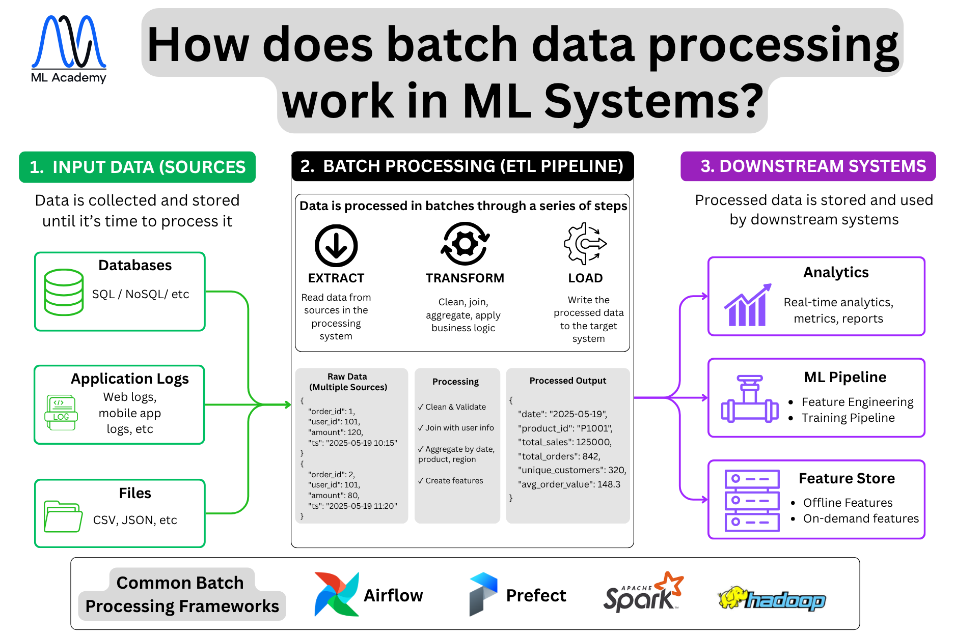
The processing follows an ETL pipeline: Extract, Transform, Load.
Extract reads data from sources into the processing system. In a demand forecasting system, this means pulling last night's sales records from Snowflake, promotion data from Salesforce, product attributes from PostgreSQL, and external data like weather and public holidays from third-party APIs.
The transform step cleans and validates these records, joins them with product and user data from other sources, then aggregates by date, product, and region to produce features the model can actually use.
This is where most of the feature engineering happens in batch systems — rolling averages over the last 7 or 30 days, lag features, sales velocity by SKU, promotional uplift calculations. None of this requires low latency, so it makes sense to compute it in bulk overnight rather than on every incoming event.
Load writes the processed output to the target system. Aggregated features go to the feature store for use during model training and batch inference. Summary tables go to the analytics platform. Training-ready datasets get written to object storage like S3 in Parquet format, where the training pipeline picks them up.
Common frameworks are Apache Airflow and Prefect for scheduling and orchestration — they define when pipelines run, in what order, and what to do on failure. Apache Spark or Hadoop handles the distributed computation when data volumes are too large for a single machine.
The contrast with streaming is straightforward: streaming processes each event as it arrives in milliseconds, while batch processes accumulate data on a schedule in minutes or hours.
Summary
Let's summarize what we covered in this lesson.
Data storage is not a one-size-fits-all decision.
- Relational databases work well for structured business data with relationships.
- Column-oriented databases are built for analytical queries over large datasets.
- Vector databases handle embeddings and similarity search.
- Key-value databases are built for instant lookups by a unique key, making them ideal for caching, session management, and leaderboards.
As for the data processing, there are two approaches - streaming and batch. Streaming processes each event within milliseconds, which is why it powers fraud detection and real-time recommendations. Batch accumulates data over time and processes it in bulk, which is the right fit for demand forecasting and overnight feature computation.
The choice between them comes down to one question: how quickly does your system need to act on new data.
These two layers sit underneath everything else in an ML system.
In the next lesson, we will go one level up and look at ML pipelines, which are the automated workflows that take data from storage, process it, and turn it into trained models.
Related Articles
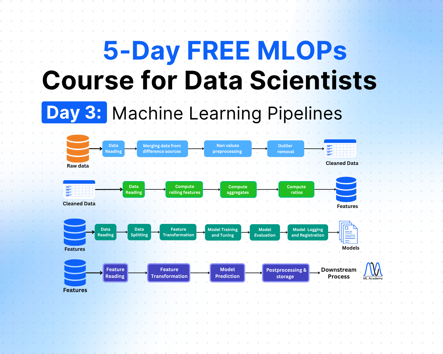

Free MLOps Course for Data Scientists: Day 3 - Machine Learning Pipelines
A practical guide to ML pipelines for Data Scientists: preprocessing, feature engineering, training, and inference pipelines explained with Python code examples and implementation best practices.
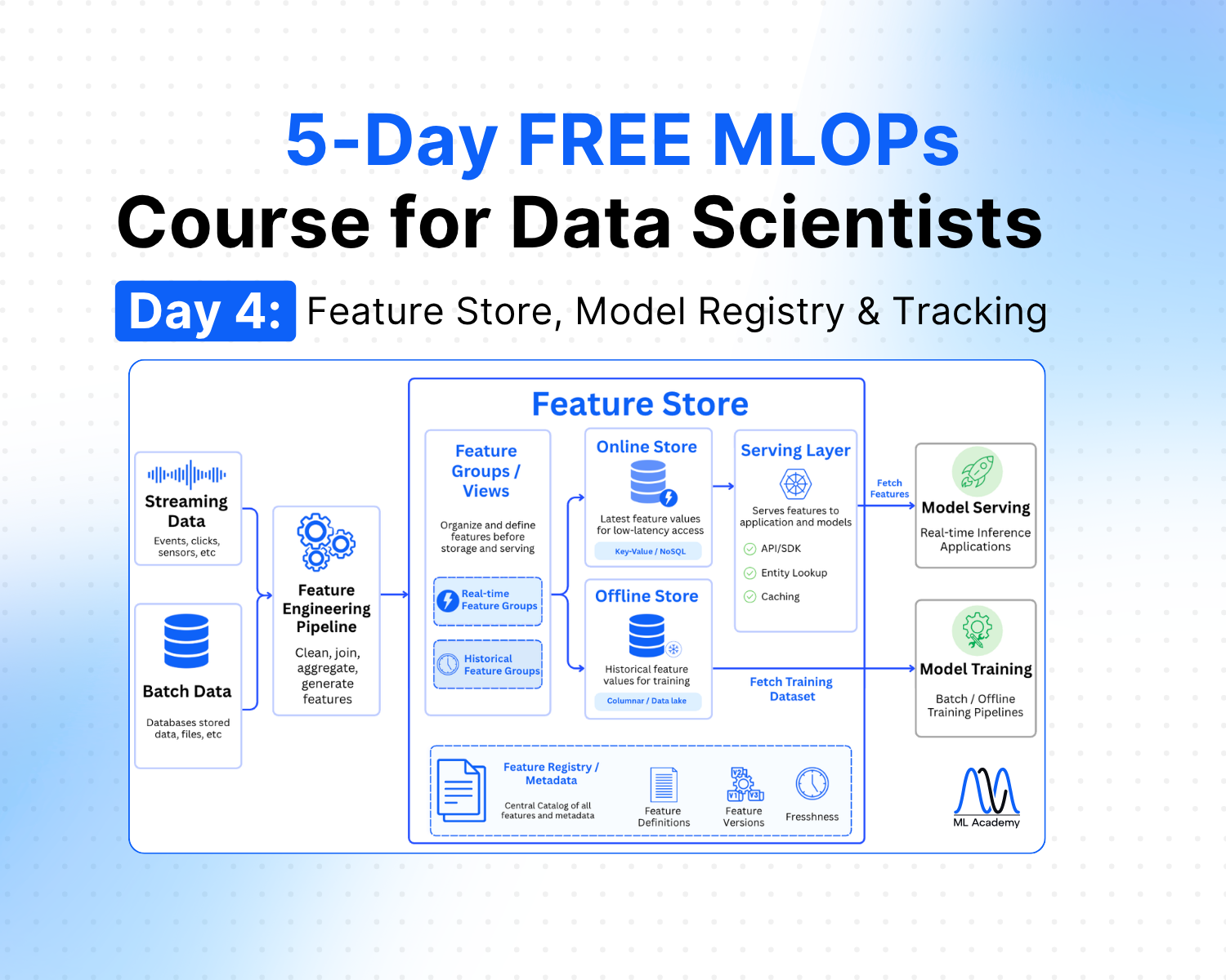
Free MLOps Course for Data Scientists: Day 4 - Feature Store, Model Registry and Experiment Tracking
A practical guide to feature stores, experiment tracking, and model registry for Data Scientists: what each component does, when to use them, and how they connect in a production ML system.
Ready to transform your ML career?
Join ML Academy and access free ML Courses, weekly hands-on guides & ML Community