Intro

The full code of the tutorial is HERE.

In Part 1 of the MLFlow experiment tracking (link), we covered the basics of MLFlow Experiment Tracking functionality, which still covers quite a lot and allows us to start working with the library efficiently.

However, in most cases, we need to go beyond logging basic entities such as parameters and metrics. Also, within 1 run, we often want to test multiple different parameters for an ML model, e.g., perform hyperparameter optimization.

In this part of the tutorial, we will cover:

- How to run many sub-runs (child runs) within a single MLflow experiment run

- How to use child runs to write hyperparameter optimization with Optuna

- How to store artifacts such as feature scalers or performance plots

What Are MLflow Parent and Child Runs?

MLflow tracks experiments as named groups where all your related runs live. As we have seen up to now, each "run" is one training session where you log parameters, metrics, and artifacts. Parent and Child Runs add a hierarchical layer to this setup.

Here's a real-world example: You're experimenting with different deep learning architectures. Instead of having all your runs jumbled together:

• Each architecture (CNN, ResNet, Transformer) becomes a parent run
• Every hyperparameter tuning iteration becomes a child run nested under its parent

Boom. Instant organization.

Here's a schematic representation of the parent and child runs based on LASSO and Catboost Baseline Model runs that we conducted in Part 1 of the tutorial.

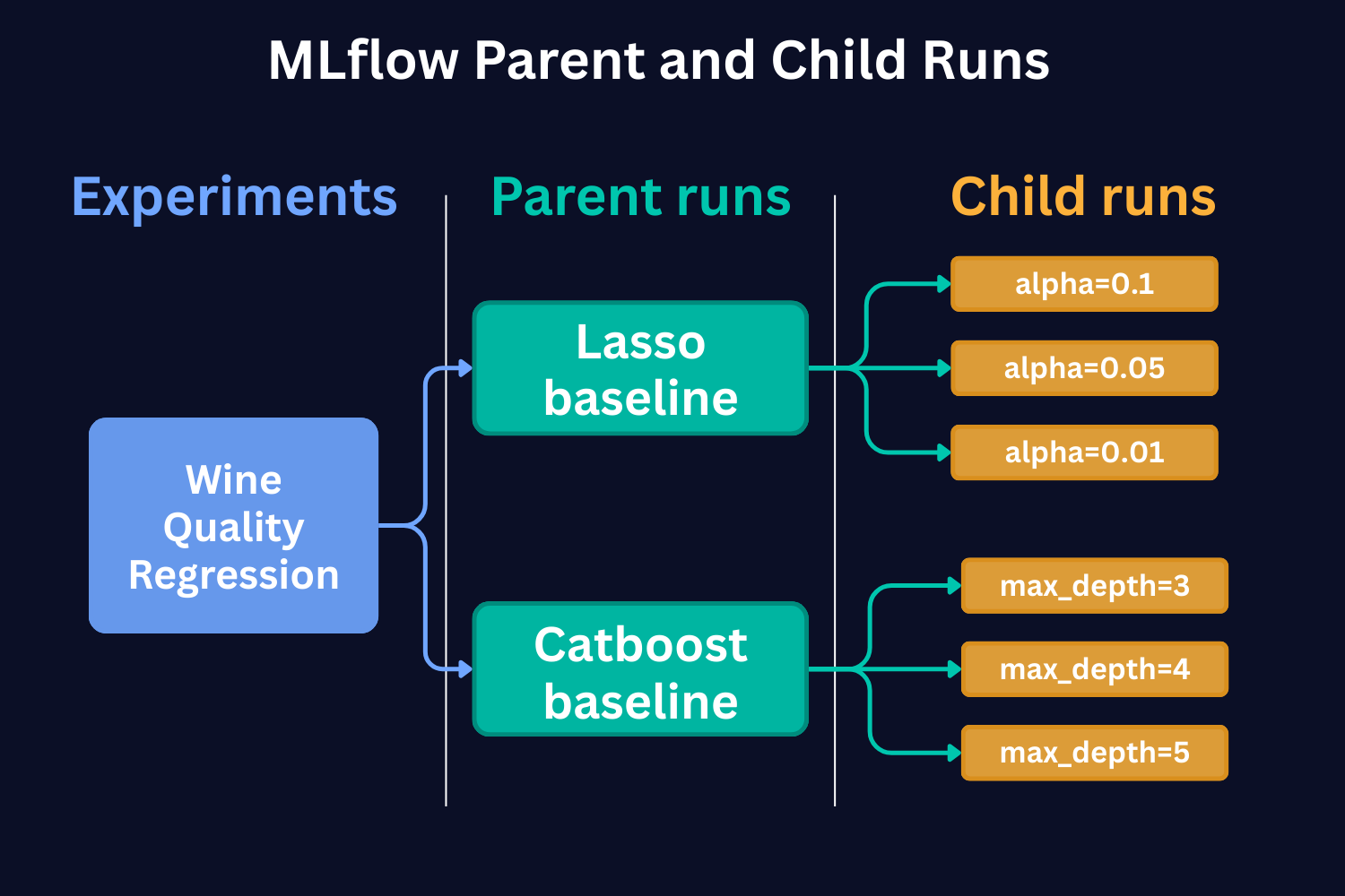
Schematic representation of Parent and Child MLflow runs

In Part 1 of the tutorial, we conducted the runs with just one set of hyperparameters. But if we were to run with different hyperparameters and compare them to each other, child runs would be the way to go. As we see from the figure above, each child run represents a single model training run with a different value of the hyperparameter.

In the case of Catboost, this would be a different SET of hyperparameters. In the figure, for the sake of simplicity, we show that each run has only a different max_depth hyperparameter.

Why Should You Care?

1. Organizational Clarity.

With a parent-child structure, related runs are automatically grouped together. When you're running a hyperparameter search using a Bayesian approach on a particular model architecture, every iteration gets logged as a child run, while the overarching Bayesian optimization process becomes the parent run. This eliminates the guesswork of figuring out which runs belong together.

2. Enhanced Traceability.

When working on complex projects with multiple variants, child runs represent individual products or model variations. This makes it straightforward to trace back results, metrics, or artifacts to their specific run configuration. Need to find that exact setup that gave you the best performance? Just follow the hierarchy.

3. Improved Scalability.

As your experiments grow in number and complexity, having a nested structure ensures your tracking remains manageable. Navigating through a structured hierarchy is much more efficient than scrolling through a flat list of hundreds or thousands of runs. This becomes particularly valuable as projects scale up.

Now, as the concept of Parent and Child runs is clear, let's see how we can implement this.

A Practical Example: LASSO Hyperparameter Tuning

Grid Search Approach

Let me show you how this works with our LASSO example. Say you're testing a LASSO model with different alpha values - from 1 to 0.001.

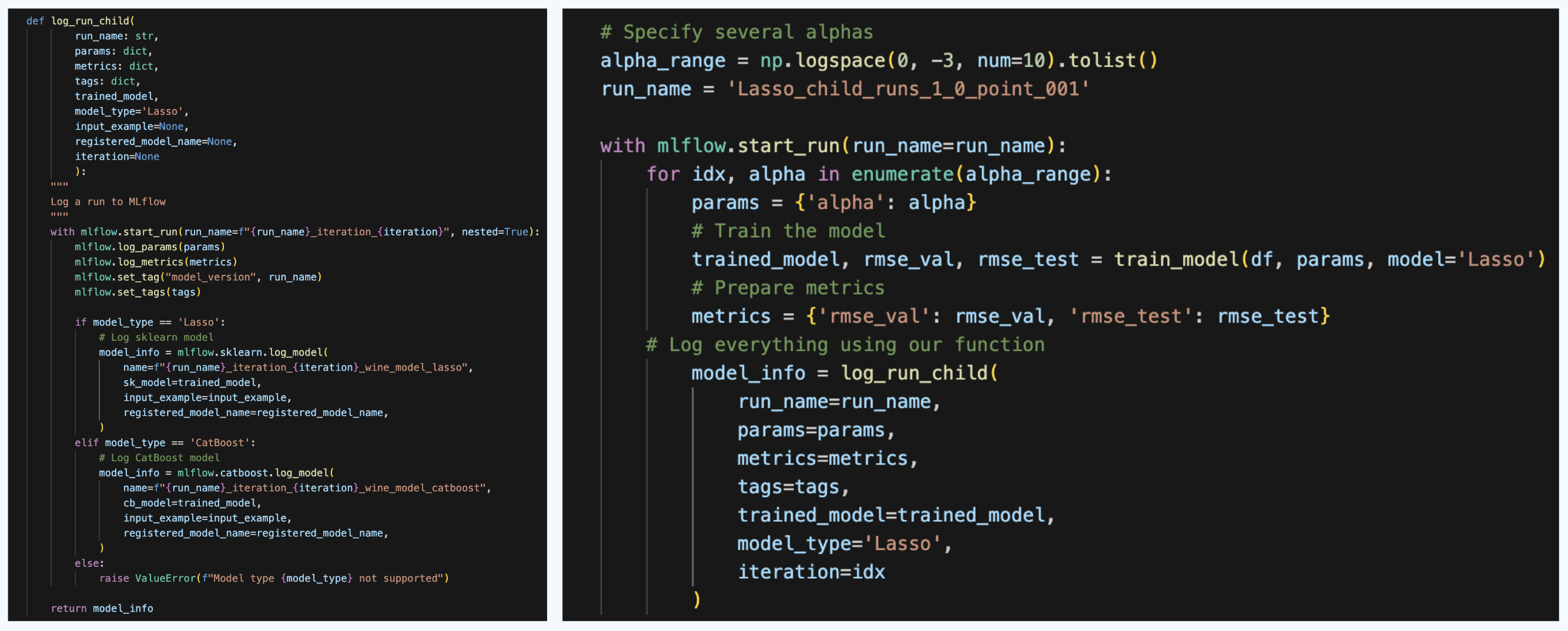
To do that, we create a function log_run_child.

This is a very similar function to log_run, but here we change the names of the run at each run and also specify parameter nested=True. This parameter indicates to MLflow that the runs are child runs.

Then we specify the parent run, and in a loop we run the child runs.

 When we run this, we get the parent and child runs in the UI. We can then select them and compare.

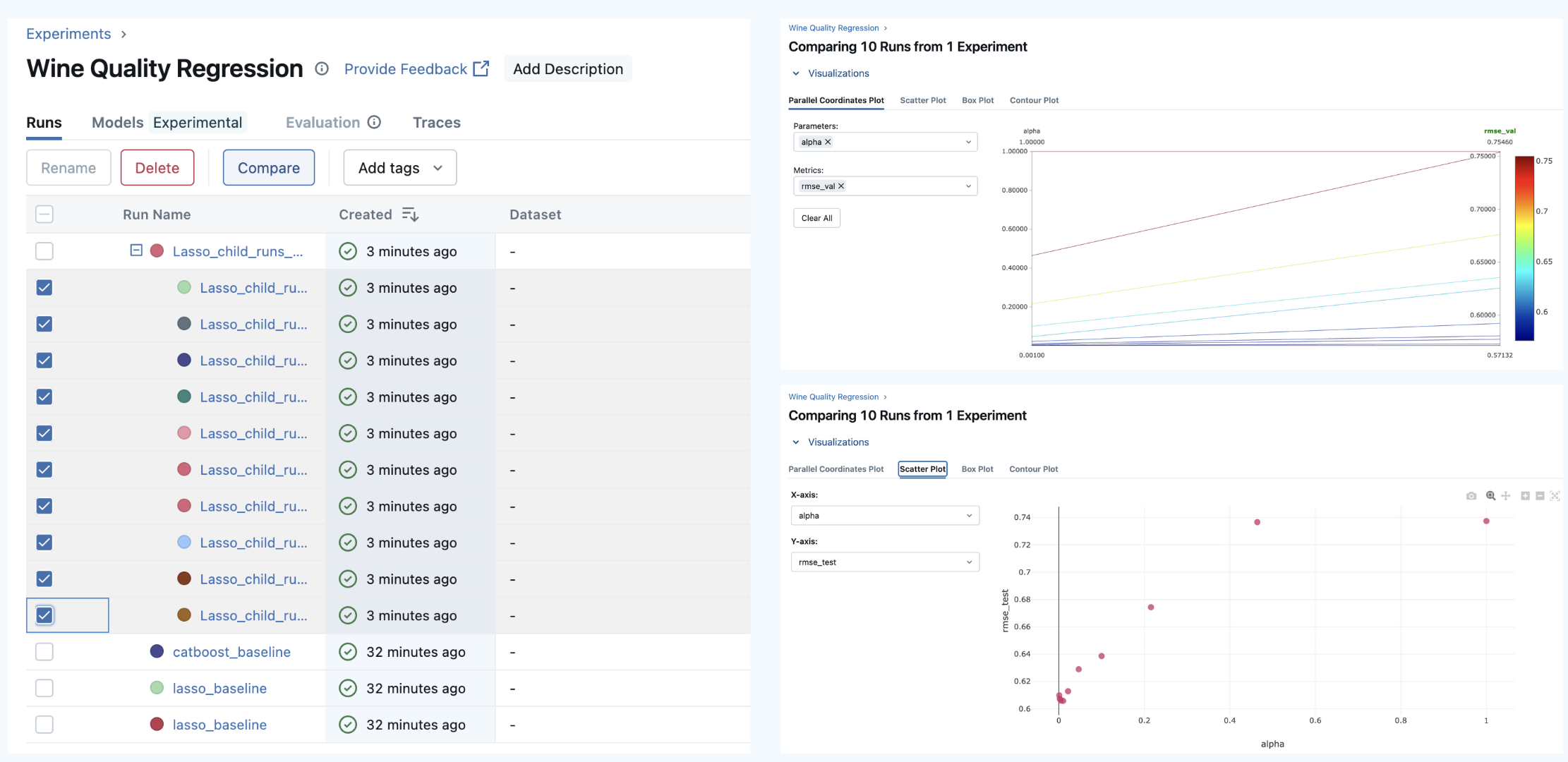 Awesome! Now, we keep our hierarchy and UI clean, make a lot of experiments, and efficiently compare them.

MLflow Child Runs with Optuna Hyperparameter Tuning

Let's now make things a little bit more complex.

Let's say we want to tune a CatBoost model and want to use Optuna library for this.

Optuna uses Bayesian Optimization under the hood in order to select the best set of hyperparameters. Let's take a quick look at how it does that.

 Bayesian Optimization is an approach to finding the minimum of a black-box function using probabilistic models to select the next sampling point based on the results of the previous samples.

Here are the main steps Bayesian Optimization takes (the gif below shows this process dynamically):

As we see, Bayesian Optimization aims to iteratively optimize the given objective function. In contrast, the two most frequent hyperparameter optimization approaches either follow the pre-specified values (Grid Search) or randomly sample the search space (Random Search).

The example below compares the three approaches. As we can see, the cumulative value of the objective function of the Bayesian Optimization is much lower and converges to some value over time. This means that the quality of samples that Bayesian Optimization performs is higher (can also be seen on the first subplot).

Note: The example below uses Hyperopt (Optuna alternative), but the idea behind it is the same.

Now, as we know a little bit about how Optuna works, let's use it with MLflow.

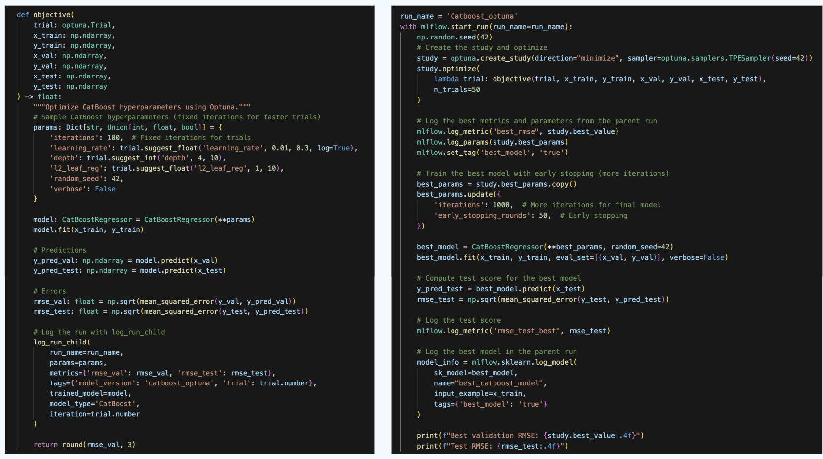
For this, we need to do two things. First, we need to define the objective function that Optuna will try to optimize. In our case, this is an error in the validation set. For the metric, we will choose RMSE. Within the objective function, we will:

• train the model
• compute the metrics on the validation set
• log the run as a child run
• return the validation RMSE error

We will run 50 Optuna trials, meaning that we will train the model 50 times and then select the best run. A good practice is to use a fixed value for the number of Gradient Boosting trees when tuning other hyperparameters. Then, finetune this number using early stopping. This is what we will do.

Finally, we will re-train the model on the entire train set (i.e., including the validation set that has been used for tuning) and compute the test set RMSE.

 After the runs, we can compare them and see the tendencies of which parameters produced us the best results:

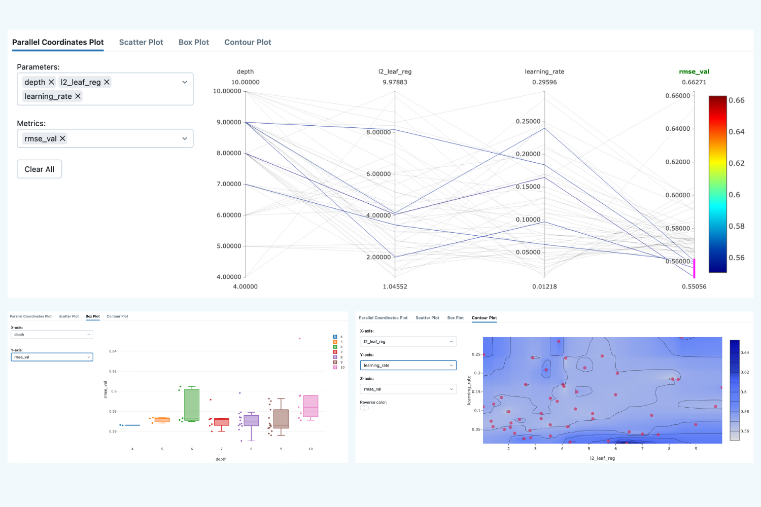
Here we see that the lowest validation scores have been produced over a wide range of hyperparameters, so it's hard to draw any valid conclusion.

Pro Tip: To make reproducible results, you need to specify the random seed in several places: in Numpy, in Optuna, and in CatBoost. See the code for the details.

Now, note that when we run the parent run, we re-train the best optuna model on the entire training set and log a tag - best_mode: true. This allows us to easily load the best model, use it for predictions and consider moving the model to production.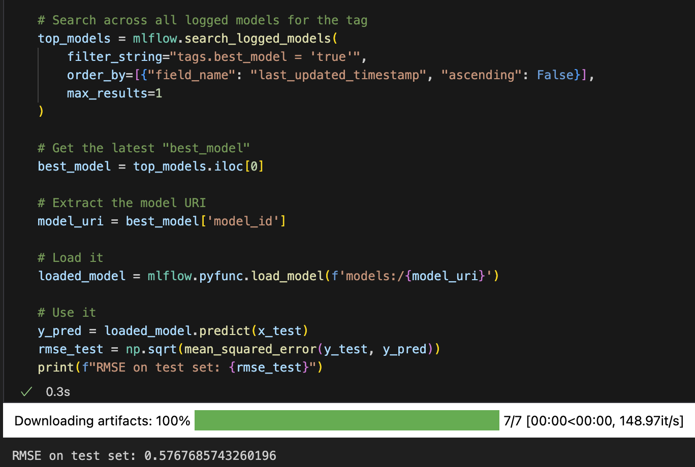

So, we have done a great job and advanced our understanding of how to run MLflow child runs using Optuna. Now, let's look at how we can log different artifacts, input model examples, and other files that are important to track and then use in the production environment.

Beyond basics - what do you need to log to MLflow?

In the examples above, in addition to the models and default metadata, we also logged model metrics and model parameters. However, this is not enough to ensure that our models are reproducible in the production environment. In the next sections, we will learn how to log some more essential data to make our ML pipelines more robust.

Model Signatures and Input Examples

Model signatures and input examples are foundational components that define how your models should be used, ensuring consistent and reliable interactions across MLflow's ecosystem.

Model Signature - Defines the expected format for model inputs, outputs, and parameters. Think of it as a contract that specifies exactly what data your model expects and what it will return.

Model Input Example - Provides a concrete example of valid model input. This helps developers understand the required data format and validates that your model works correctly.

Why Signatures Matter

1. Validation → When you load the model, MLflow checks if the provided data matches the signature.

2. Serving → If you deploy via MLflow Model Serving, the API auto-generates schemas based on the signature.

3. Reproducibility → Clear documentation of what the model expects.

4. Portability → Makes it easier to share models across teams.

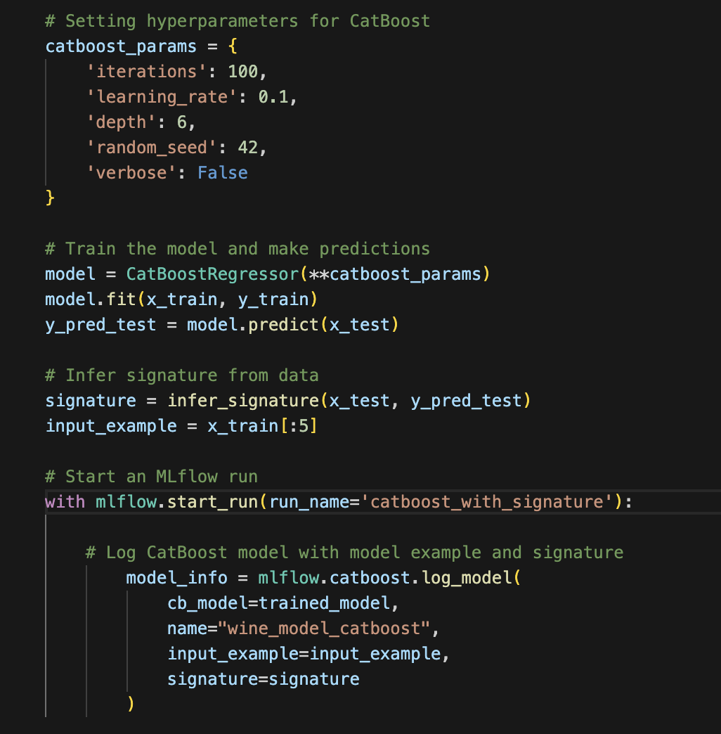
MLflow allows us to easily log signatures and input examples. Below, you see that we can infer the signatures from our data using the infer_signature helper and then log it using log_model method together with the input example.

Logging artifacts

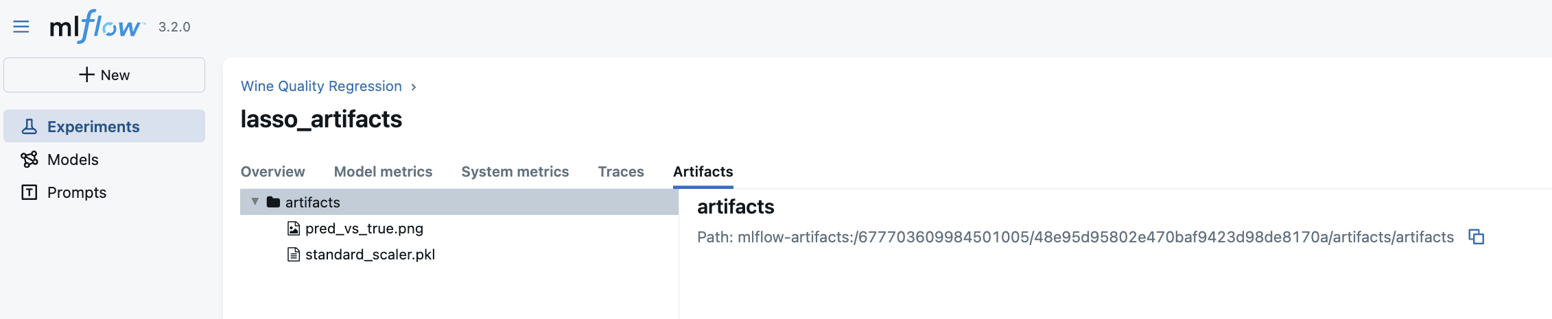
In addition to the model artifact that is logged by default, we can also log other artifacts, such as feature scalers, plots, or other useful files. Let's make an example with a Lasso model, a standard scaler, and a prediction plot.

Awesome! Now, we can access artifacts both programmatically and from the User Interface.

That is it for this part of the tutorial! In the next part, we will consider the MLFlow Model registry concept, how to register the models both programmatically and from the UI, and how to use tags and aliases to make it handy.