Introduction to MLflow Experiment Tracking

One inevitable part of the daily work of a Data Scientist is to build ML models. However, you rarely come up with a good model from the very beginning. Usually, creating a good model takes a lot of effort and experiments.

In my career, I have conducted thousands of experiments, if not tens of thousands. And a very common issue with experiments is that you quickly get lost in them.

What was the feature setup that gave me the best score? Did I scale data for that experiment? What were the resulting hyperparameters? What about the search space that I used for the learning rate? Do I even remember what the score was?

These questions appear all the time. I am sure you have been there, and you are not alone, trust me.

If there is a problem, usually there is a solution. And there is a solution created for experiment tracking. In fact, there are many of them.

The most common framework/library for experiment tracking (and, in fact, for the full model management lifecycle) is MLflow. It was one of the first tools (maybe even the first one) in the community that aimed to solve problems with experiment tracking and ML model management.

In this article, we will learn:

• What is the idea behind Experiment Tracking in general
• What MLflow is
• What components does it have
• How to start using MLflow for tracking ML experiments.
• How to select the best ML model from these experiments.

In the following articles, we will also consider how to push ML models to a Model Registry from which you can then serve models to the inference stage of your ML pipelines.

 

What is ML Experiment Tracking?

Here's how I formulate experiment tracking: 

Logging and tracking all the important stuff about your ML experiments so you don't lose your mind trying to remember what you did.

Every time you train a model, a good experiment tracker captures:

• The exact code you ran (Git commits, scripts, notebooks)
• All your hyperparameters and configurations
• Model metrics
• Model weights/files.
• What data did you use, and how did you process it
• Your environment setup (Python versions, packages, etc.)
• Charts and visualizations (confusion matrices, learning curves, etc.)

Instead of having this information scattered across your laptop, three different cloud instances, and that one Colab notebook you can't find anymore, everything lives in one organized place.

Here's how an experiment tracking server comes into play in the ML Lifecycle. When your workflow is done right, you can link your tracking system with the model registry to be able to push the best model to production. But more importantly, you can track your choice back in any point in time, which is crucial in real-world ML deployments. Things WILL go wrong, but you just need to be prepared.

 

Main ML Experiment Tracking Use Cases

After building 10+ industrial ML solutions (while not in all of them using experiment tracking - sad face), I have found the following 4 major use cases for using experiment tracking.

1. All Your ML Experiments in One Place

I just like things to be organized. I believe you do it too.

I have several projects where my team and I did NOT use experiment tracking. The result is that the team had their own experiments locally, and it was just very hard to compare them. Not good.

On the other hand, with experiment tracking, all your experiment results get logged to one central repository.

It does not matter who, where, and how they run them; they are just there. Waiting to be analyzed to help you make money with your ML models.

You don't need to track everything, but the things that you track, you know where to find them.

This makes your experimentation process so much easier to manage. You can search, filter, and compare experiments without remembering which machine you used or hunting through old directories.

2. Compare Experiments and Debug Models with Zero Extra Work

When you are looking for improvement ideas or just trying to understand your current best models, comparing experiments is crucial.

Modern experiment tracking systems make it quite easy to compare the experiments.

What I also like a lot is that you can visualize the way the model/optimizer tends to select hyperparameters. It can give you an idea of what the model is converging to.

From there, you might come up with ideas of how the model can be further improved. 

3. Better Team Collaboration and Result Sharing

This point is connected to Point 1.

Experiment tracking lets you organize and compare not just your own experiments, but also see what everyone else tried and how it worked out. No more asking "Hey, did anyone try batch size 64?" in Slack.

Sharing results becomes effortless too. Instead of sending screenshots or "having a quick meeting" to explain your experiment, you just send a link to your experiment dashboard. Everyone can see exactly what you did and how it performed.

 

Experiment tracking as the central place between Data Scientists and the Model Registry

4. Monitor Live Experiments from Anywhere

When your experiment is running on a remote server or in the cloud, it's not always easy to see what's happening.

This is especially important when you are training Deep Learning models.

Is the learning curve looking good? Did the training job crash? Should you kill this run early because it's clearly not converging?

Experiment tracking solves this. While keeping your servers secure, you can still monitor your experiment's progress in real-time. When you can compare the currently running experiment to previous runs, you can decide whether it makes sense to continue or just kill it and try something else.

 

Main components of MLflow experiment tracking

MLflow experiment tracking is a component of the MLflow framework that is responsible for logging parameters, code versions, metrics, and output files when running your machine learning code and for later visualizing the results. MLflow Tracking lets you log and query experiments using Python, REST, R API, and Java API APIs.

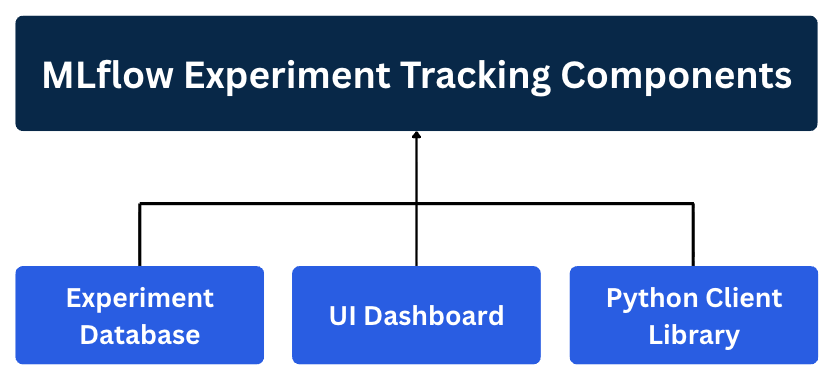
In general, the MLflow tracking system can be split into 3 main components:

1. The Database (Experiment Memory)

This is where all your experiment metadata gets stored. It's usually a local file system or a cloud-based database that can handle structured data (metrics, parameters) and unstructured data (images, model files, plots).

2. The Client Library (Logging Python Library)

This is the Python library you integrate into your training code. Combined with ML Tracking Server processes, it's what actually sends your experiment data to the database.

 

3. The Web Dashboard (User Interface)

This is the web interface where you visualize, compare, and analyze all your experiments. This component makes it convenient to take a closer look at your result and draw conclusions about which parameters or models are best to choose for the deployment and what parameter trends are with respect to the model accuracy (e.g., you can answer the question: "Do deeper Gradient Boosting trees give better scores for the particular dataset?").

 

What exactly does MLflow store?

There are 2 main data types that MLflow stores:

1. MLflow entities - model parameters, metrics, tags, notes, runs, metadata. The entities are stored in a backend store.

2. Model artifacts - model files, images, plots, etc. The artifacts are stored in artifact stores.

There are different ways in which these 2 data object types are stored and how the Python Client library can be used. The MLflow documentation describes 6 main scenarios.

In this article, we will cover the 2 most common ones (Scenario 3 and 4 in the documentation). Reading the documentation can be useful, but below we will make things clearer than they are described in the documentation, so please, follow along!

 

Scenario 1 (Scenario 3 in docs) - MLflow on localhost with Tracking Server

In this scenario, a Data Scientist stores all the files locally in the machine on which he runs the code. The figure below schematically shows this approach.

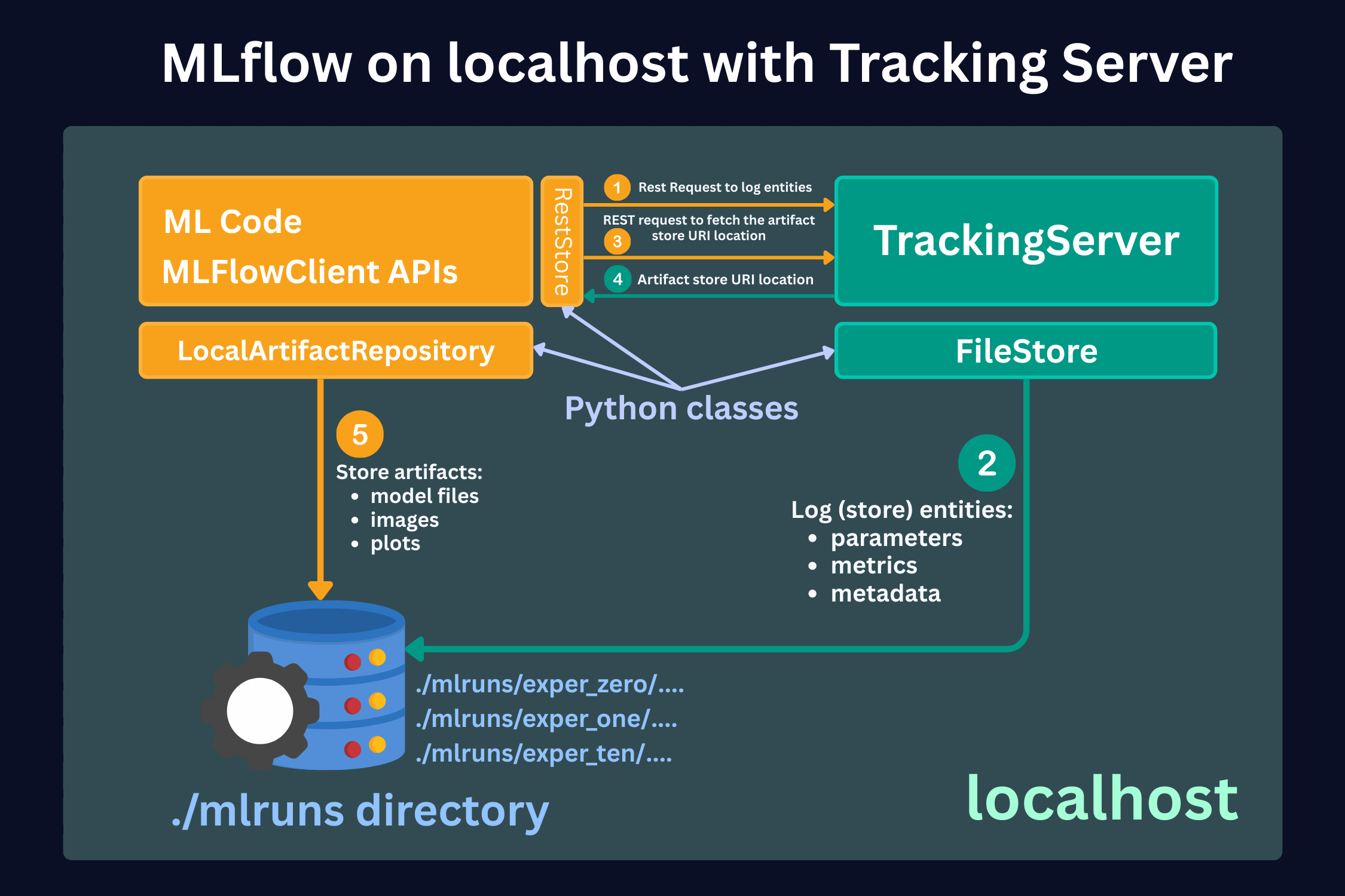
Schematic representation of the MLflow file storing process when running locally with a Tracking Server

Here, we see 3 main parts:

1. ML code and MLFlowClient APIs (yellow box).

This is where you run your code and make experiments. Here, by using MLFlow Library Python Class RestStore, you can communicate with a Tracking Server (more on it below), which tells you what the URI (Uniform Resource Identifier, e.g., users:/alex/mlruns/) is where the artifacts are stored.

In case of storing it locally, this is a folder somewhere on your machine. By default, this is the folder ./mlruns in the directory where you run your code.

When the MLFlowClient gets this information, it then uses the LocalArtifactRepository class to store the artifacts (files) in this directory (blue database image).

2. Tracking Server (green box).

Tracking Server is a running process on your local machine (by the way, you can see that all the boxes are inside a green shadow box, which describes localhost - your local machine). This Server (process) communicates with the MLFlowClient through REST requests (as described above) to supply the required information for the artifact storage.

What it also does is it uses the FileStore Python class to store the entities (parameters, metrics, metadata, etc.) in the local storage directory (mlruns folder).

3. Local Data Store (blue database icon)

In this scenario, this is just your local directory, which is by default created in the directory where you run your code. Here, the folder mlruns is created, where both artifacts (models) and entities (metadata) are stored.

 

What is a typical use case for this local storage setup?

This setup is often used when Data Scientists run their experiments locally and do not bother with sharing the results with their team members. Also, in this case, you need to set up a separate process to send the resulting model to the deployment infrastructure. In the worst case, you should also upload the model manually.

Pros:

- Quick setup, no infrastructure required

- User does not need any knowledge of the remote storage setup

Cons:

- Hard to share results with other team members

- Hard to deploy the selected models

 

Scenario 2 (Scenario 4 in docs) - MLflow with remote Tracking Server, backend, and artifact stores

In this case, you still run your experiments locally. However, the Tracking Server, the artifact store, and the backend store are running on remote servers, e.g., on AWS.

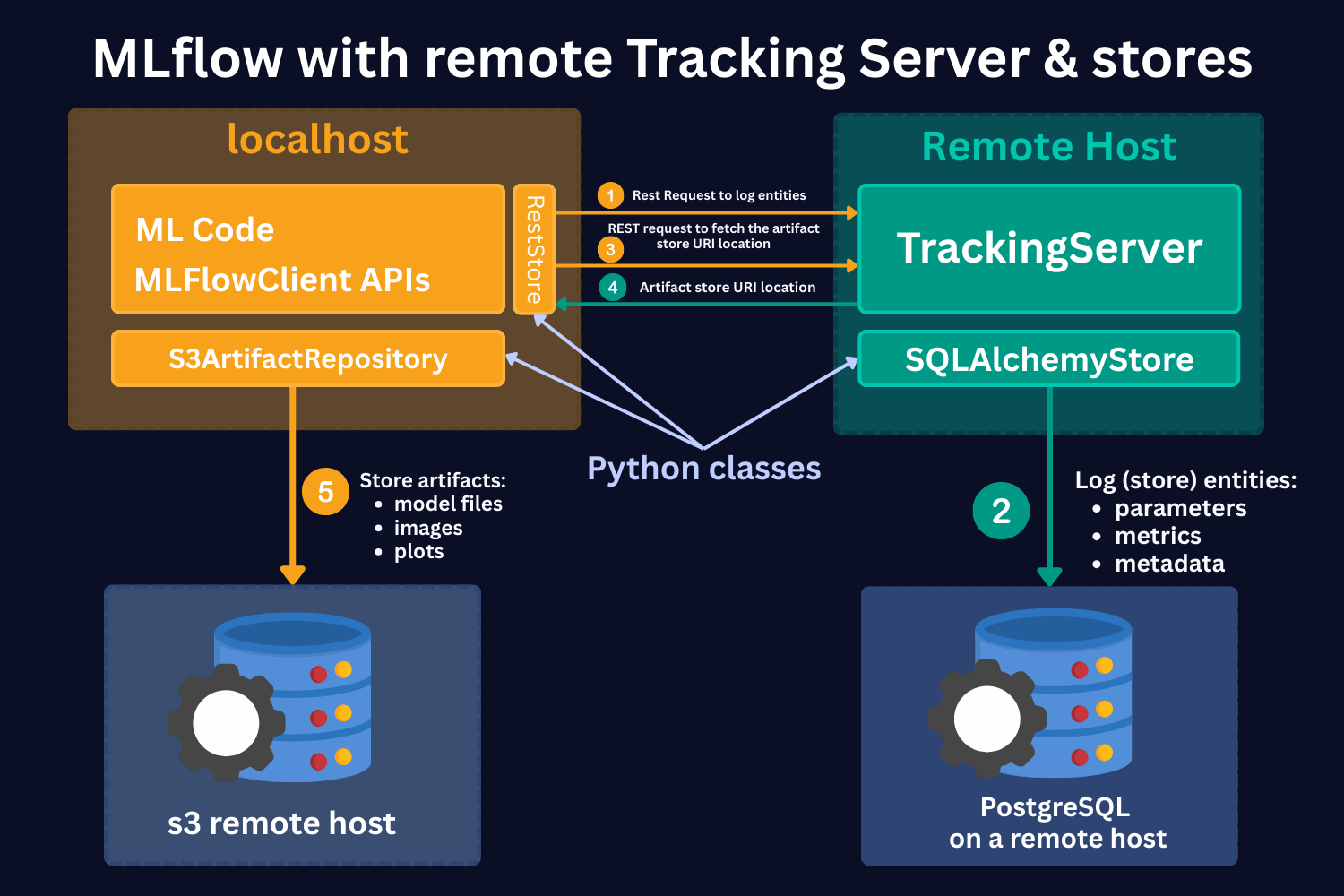
Schematic representation of the remote (cloud) MLflow file storing process with a Tracking Server running remotely

Here, we see the same 4 main parts:

1. ML code and MLFlowClient APIs (yellow box).

As in the local case, by using MLFlow Library Python Class RestStore, you can communicate with a Tracking Server (more on it below), which tells you what the URI (Uniform Resource Identifier) is where the artifacts are stored.

However, in this case, you store artifacts on the S3 remote host (as an example). Note that it should not necessarily be an S3 store. It can be any other remote storage location, for instance, Azure Blob storage.

In case of S3 bucket storage, MLflow uses the s3ArtifactRepository class to store artifacts.

2. Tracking Server (green box).

Tracking Server is a running process on a remote host. This Server (process) communicates with the MLFlowClient through REST requests (as described above) to supply the required information for the artifact storage.

It also stores the mlruns entities. However, in this case, it uses the SQLAlchemyStore class to communicate with SQL-like remote databases, for instance, PostgreSQL.

3. S3 remote host Data Store (left-hand side blue database icon).

This is a remote store for mlruns artifacts. As mentioned, this should not necessarily be S3 buckets. It can be any remote/cloud-based storage system.

4. PostgreSQL remote host Data Store (right-hand side blue database icon).

This is a remote storage for mlruns entities. This is an SQL-like database, for instance, PostgreSQL or SQLite.

 

Hands-on Example (full code of the example is here)

Important Concepts of MLflow

Before starting with the code, let's introduce some important concepts.

Runs

MLflow Tracking is organized around the concept of runs, which are executions of some piece of data science code, for example, a single python train.py execution. Each run records metadata (various information about your run, such as metrics, parameters, start and end times) and artifacts (output files from the runs, such as model weights, images, etc).

Models

Models represent the trained machine learning artifacts that are produced during your runs. Logged Models contain their own metadata and artifacts similar to runs.

Experiments

Experiments group together runs and models for a specific task. You can create an experiment using the CLI, API, or UI. The MLflow API and UI also let you search for experiments.

Running the first MLflow experiment

Now, let's see how it works in practice.

To see the implementation of MLflow experiment tracking in practice, we will build ML models and conduct different experiments on a simple Wine Quality Dataset.  It contains measurements of common chemical properties—like acidity, alcohol, sulfur content, and density—for both red and white Portuguese “Vinho Verde” wines, along with a quality rating. It features 11 numeric input variables, a wine type identifier, and a quality score

The dataset has just 1,143 rows and 12 features, so we can run our experiments quickly and test different MLflow features efficiently.

In this tutorial, we will use Scenario 1 from the discussion above. We will run our experiments and their results locally, and we will use the Tracking Server to store experiment entities.

Again, the full code of the tutorial is available here.

The first thing that we need to do is to start the ML Tracking Server. To do that, in the terminal, navigate to the notebook folder and run in the terminal (command line):

mlflow server --host 127.0.0.1 --port 8080 

This is what it does:

1. Starts the MLflow Tracking Server
   A dedicated process that manages and serves your MLflow experiments.
   
   
2. Provides a Web UI
   Accessible at http://127.0.0.1:8080 (or localhost:8080), where you can browse experiments, runs, parameters, metrics, and artifacts.
   
   
3. Exposes a Tracking API Endpoint
   Other scripts or notebooks can log directly to this server if you run mlflow.set_tracking_uri("http://127.0.0.1:8080") in the code.
   
   
4. MLflow automatically creates a folder mlruns/ and mlartifacts/ in your working directory.
   Inside mlruns/, it creates subfolders for:
   1. each experiment (default is 0)
   2. each run within that experiment 

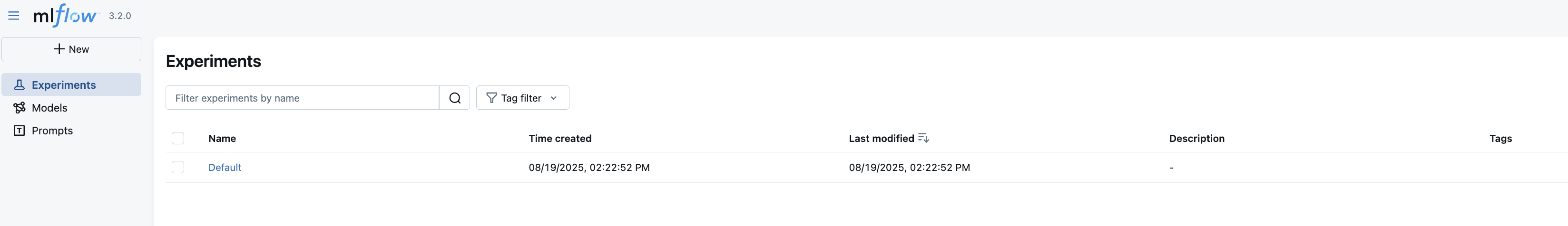
Now, if we go to  http://127.0.0.1:8080, we can see an MLflow UI with the default experiment created with no runs because we have not created any runs yet.

Before we create our first experiment, in the notebook, we set the tracking URI by running the command:

mlflow.set_tracking_uri(uri="http://127.0.0.1:8080").

What it does:

1. It tells your MLflow client (your script/notebook) where to send all logging data (experiments, runs, params, metrics, artifacts).

2. Since our host is local, it will still write to mlruns locally, but here you can configure a remote host URI.

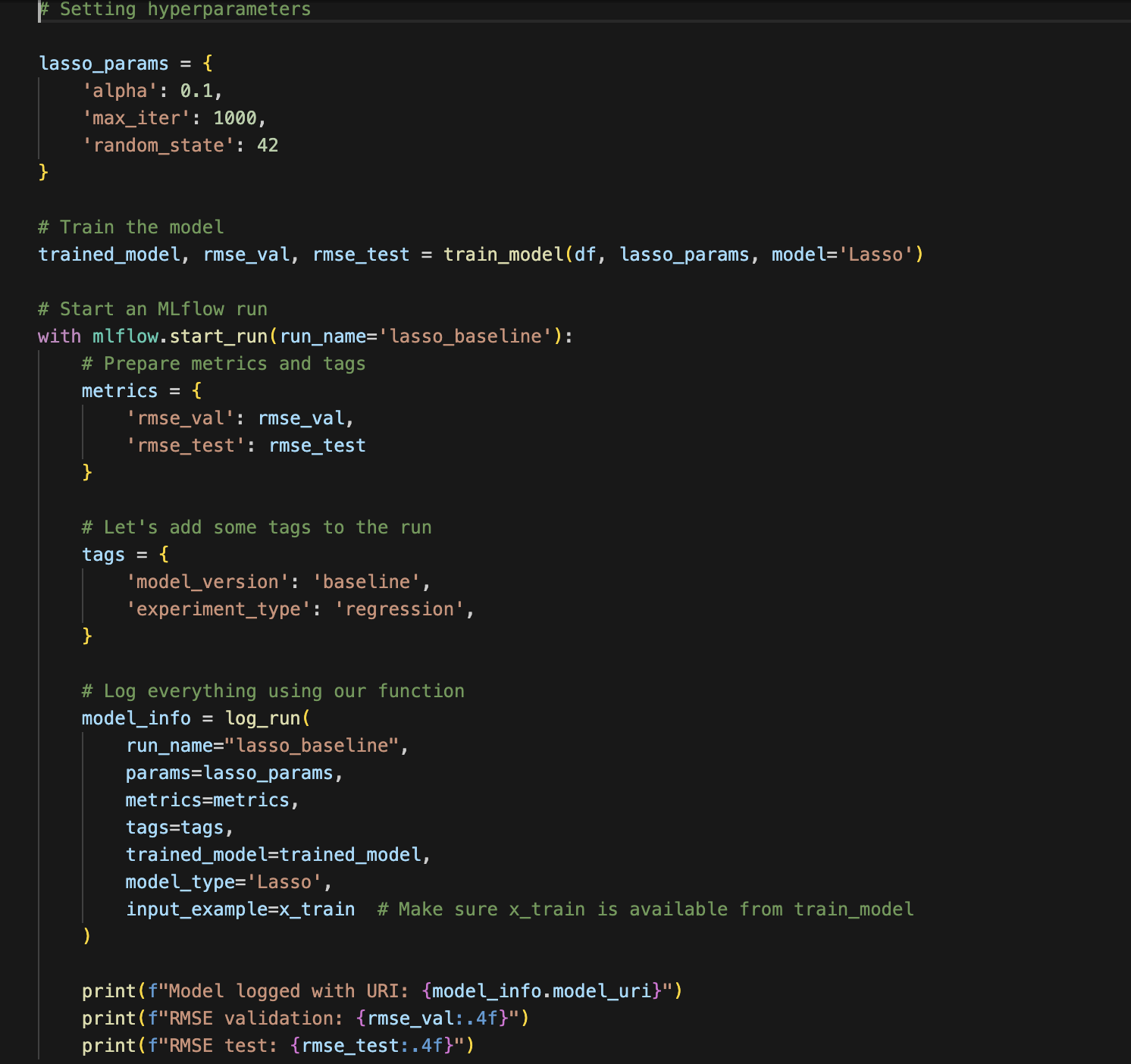
Then, we read the data, split it into training, validation, and test sets, and train a simple LASSO model with a regularization hyperparameter of alpha = 0.1.

 

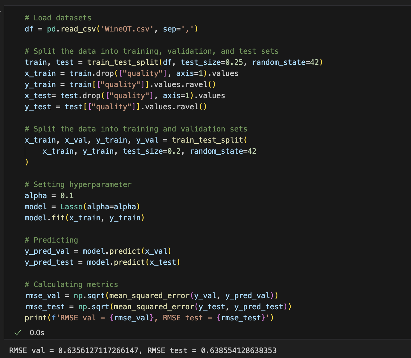
What we have just done is we conducted an experimental run! We set a hyperparameter, trained a model, and got validation and test scores (happy face). Now, our job is to log this to MLflow.

To do that, we need to run the command:

mlflow.set_experiment("Wine Quality Experiment")

If we do so, in the UI (http://127.0.0.1:8080), we will see that the experiment is created.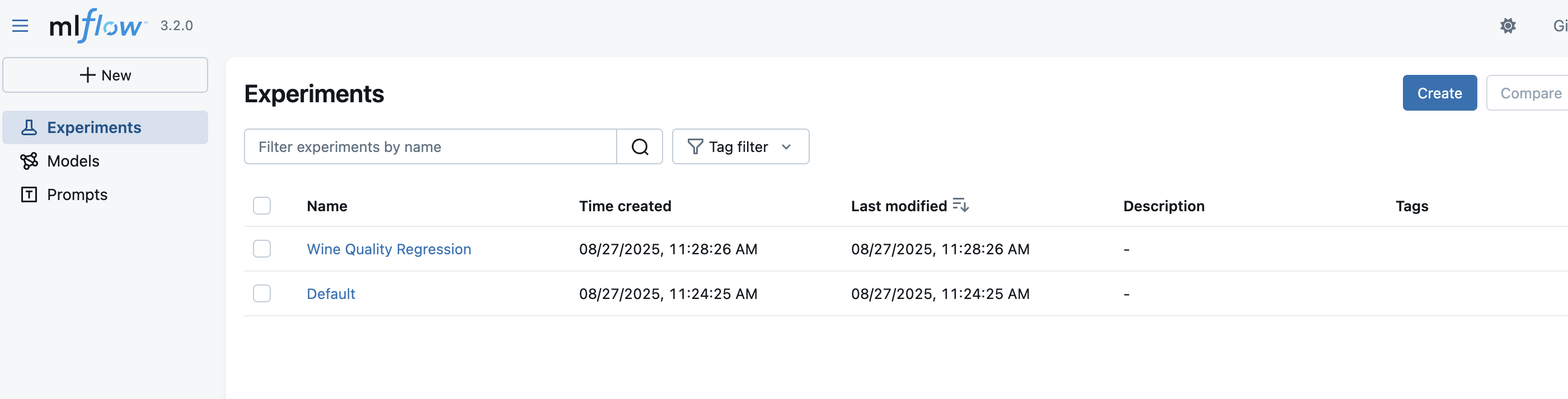

Now, all we need to do is log the parameters, metrics, and the model. Here is the full code:

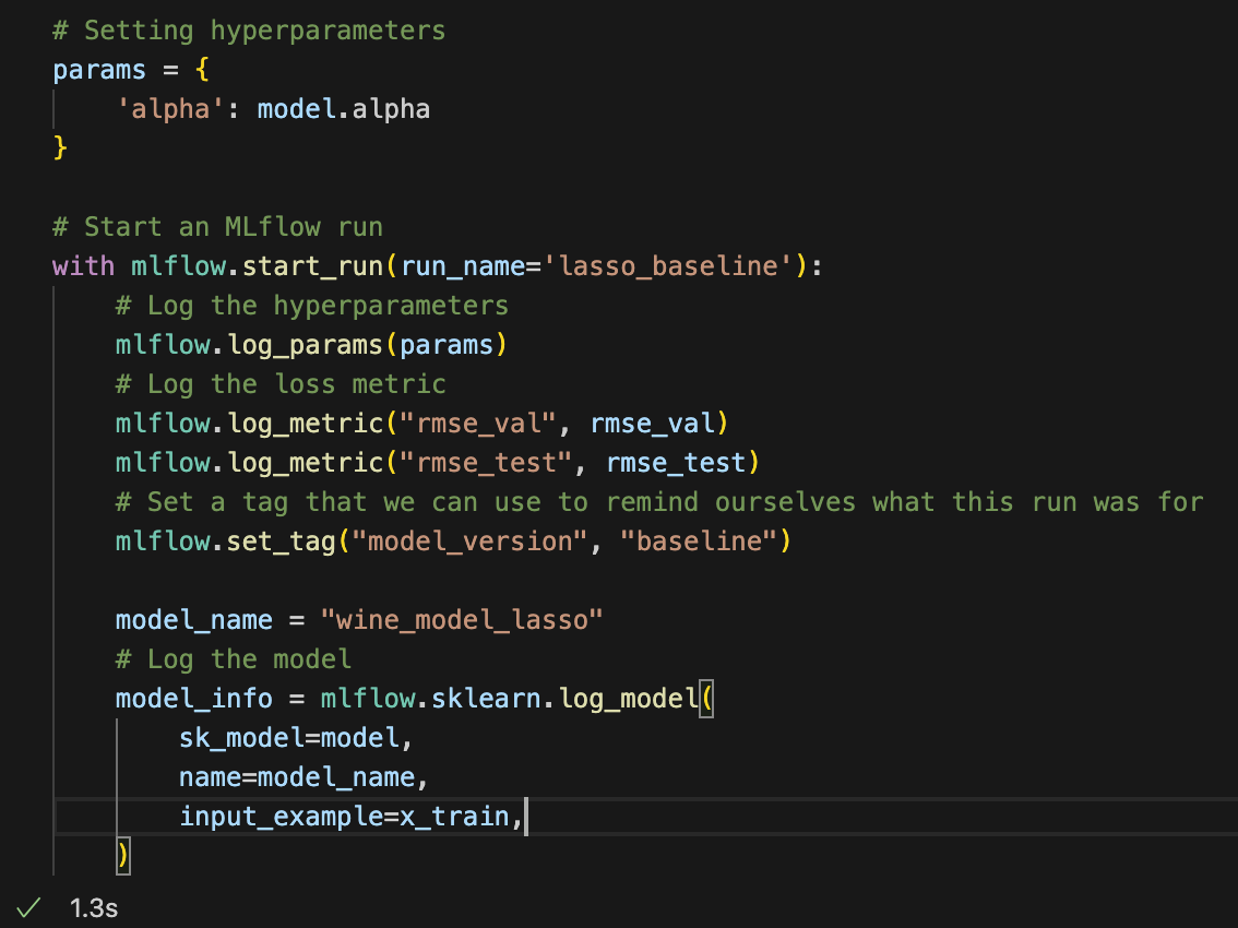
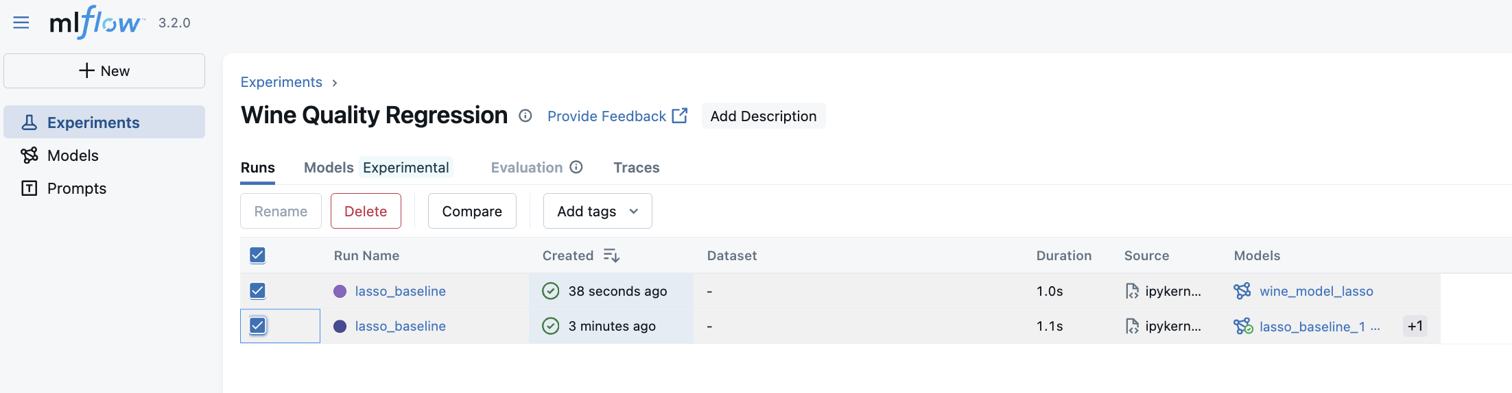
Now, in the UI, we can see that our ml run is logged!

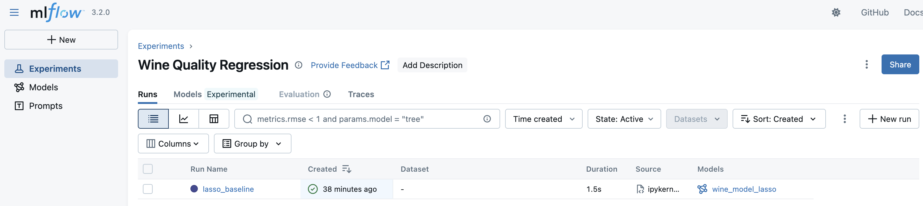
We can see the name of the model "wine_model_lasso" which we specified in the code above. Now, if we click the run, we can see more information about it.

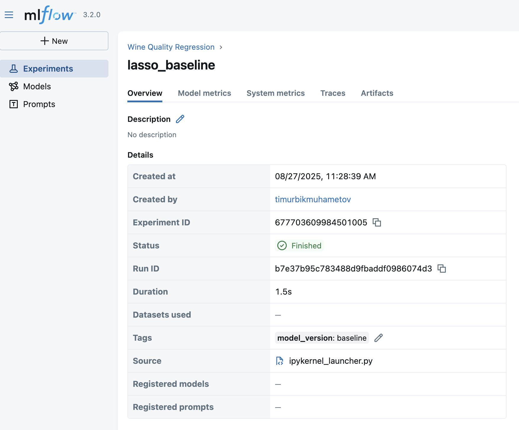
Here are some details to notice:

🔹 Metadata (Run Details)

1. Run name: lasso_baseline → descriptive name helps identify what this run was about.

2. Experiment ID & Run ID: unique identifiers that make runs reproducible and traceable.

3. Created by: the user who launched it.

3. Source: points to the script/notebook used (ipykernel_launcher.py).

Why it matters: Always give runs meaningful names and tags (model_version: baseline) so you can find them later when comparing models.

🔹 Tags

model_version = baseline

Why it matters: Tags are a simple but powerful way to label runs (e.g., baseline, tuned, production_candidate). This makes searching and filtering much easier when you have hundreds of runs.

🔹 Parameters and metrics

We see all the parameters and metrics that we logged. This will then help us to understand the model performance for the specific set of hyperparameters if we need to use it.   

Along with parameters and metrics, MLflow automatically saves artifacts from each run. 

 

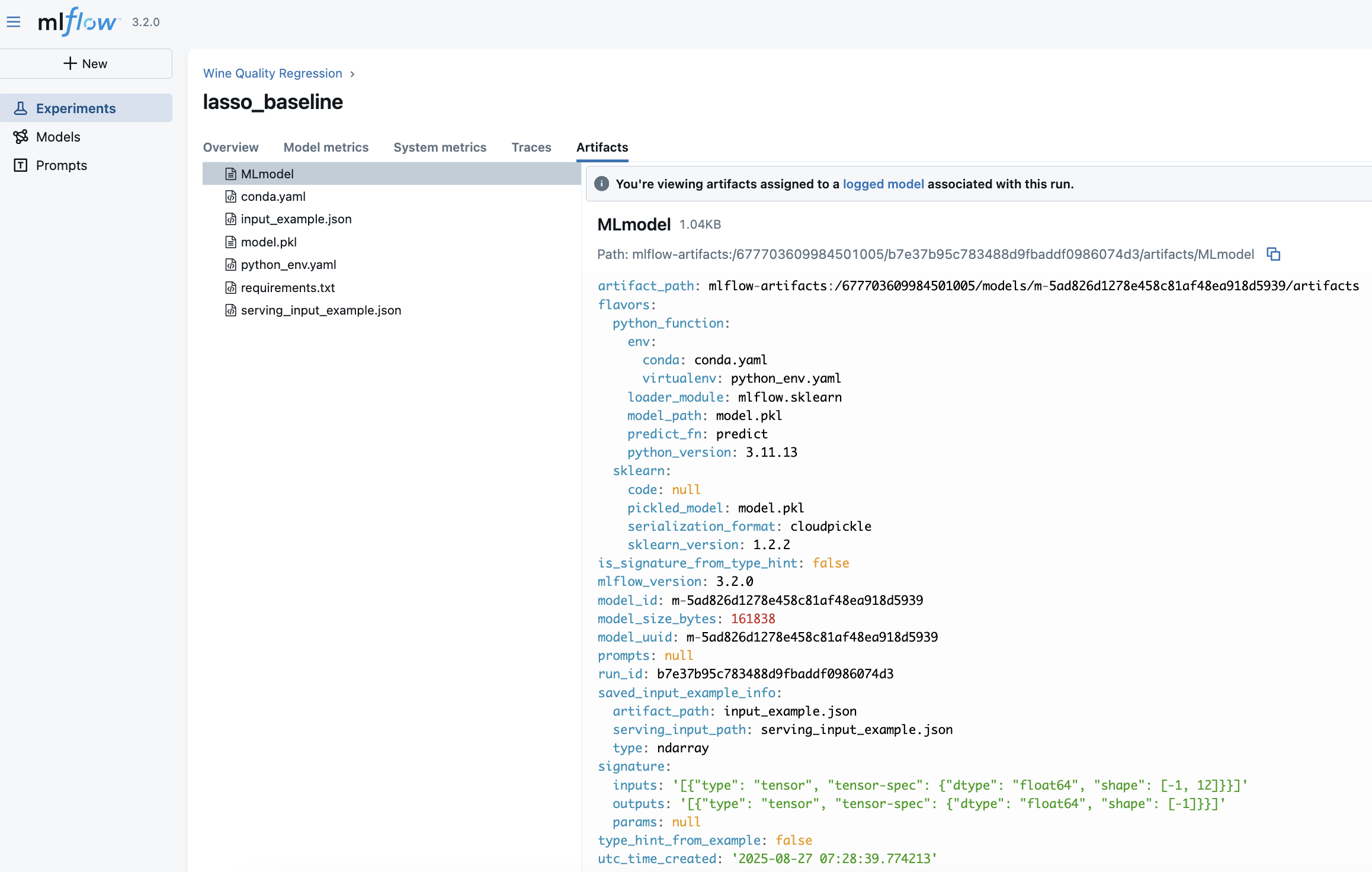
In this run (lasso_baseline), we log the following artifacts:

• MLmodel
  A metadata file that defines how to load and use the model. This file is critical - it les MLflow reload the model consistenly across environments.

  • Describes the model “flavors” (python_function for universal loading, sklearn for framework-specific).

  • Points to the environment files (conda.yaml, python_env.yaml).

  • Specifies how predictions should be made (predict_fn).

• model.pkl
  The serialized scikit-learn Lasso model — the actual trained object you can load back into Python.

• conda.yaml / python_env.yaml / requirements.txt
  Captures dependencies (Python version, libraries, package versions). These ensure reproducibility and eliminate “works on my machine” issues.

• input_example.json / serving_input_example.json
  Example input data for the model. This is useful for serving, validation, and making sure consumers know the expected input format.

Note that MLflow assigns every logged model a unique identifier, which we see in the MLmodel file - model_id and model_uuid

• This UUID is globally unique for that model instance.

• It guarantees that even if two models share the same name (e.g., lasso_baseline), MLflow can still distinguish them.

• The UUID stays constant for the life of that model version and also appears inside the artifact_path, making the model traceable back to the exact run and experiment that produced it.

In production, we'll deploy by model ID/UUID, not just by name, to avoid ambiguity if new versions are created.

Autolog

In the example above, we logged the parameters manually. However, in MLflow there is Auto-logging functionality. This feature allows you to log metrics, parameters, and models without the need for explicit log statements - all you need to do is call mlflow.autolog() before your training code. Auto-logging supports popular libraries such as Scikit-learn, XGBoost, PyTorch, Keras, Spark, and more.

In this tutorial, we will not use autolog because I want to show you all the steps as clearly as possible.

Also, while autolog seems like a nice feature, it has a big caveat. Often, you run a lot of experiments, but you don't want to log them all because some of them are just quick trials. On top, if you log all the experiments and runs, the Tracking Server UI can become messy very quickly. Personally, I rarely use auto-logging for serious projects, but it’s definitely a feature to know about and can be very convenient in the right context. 

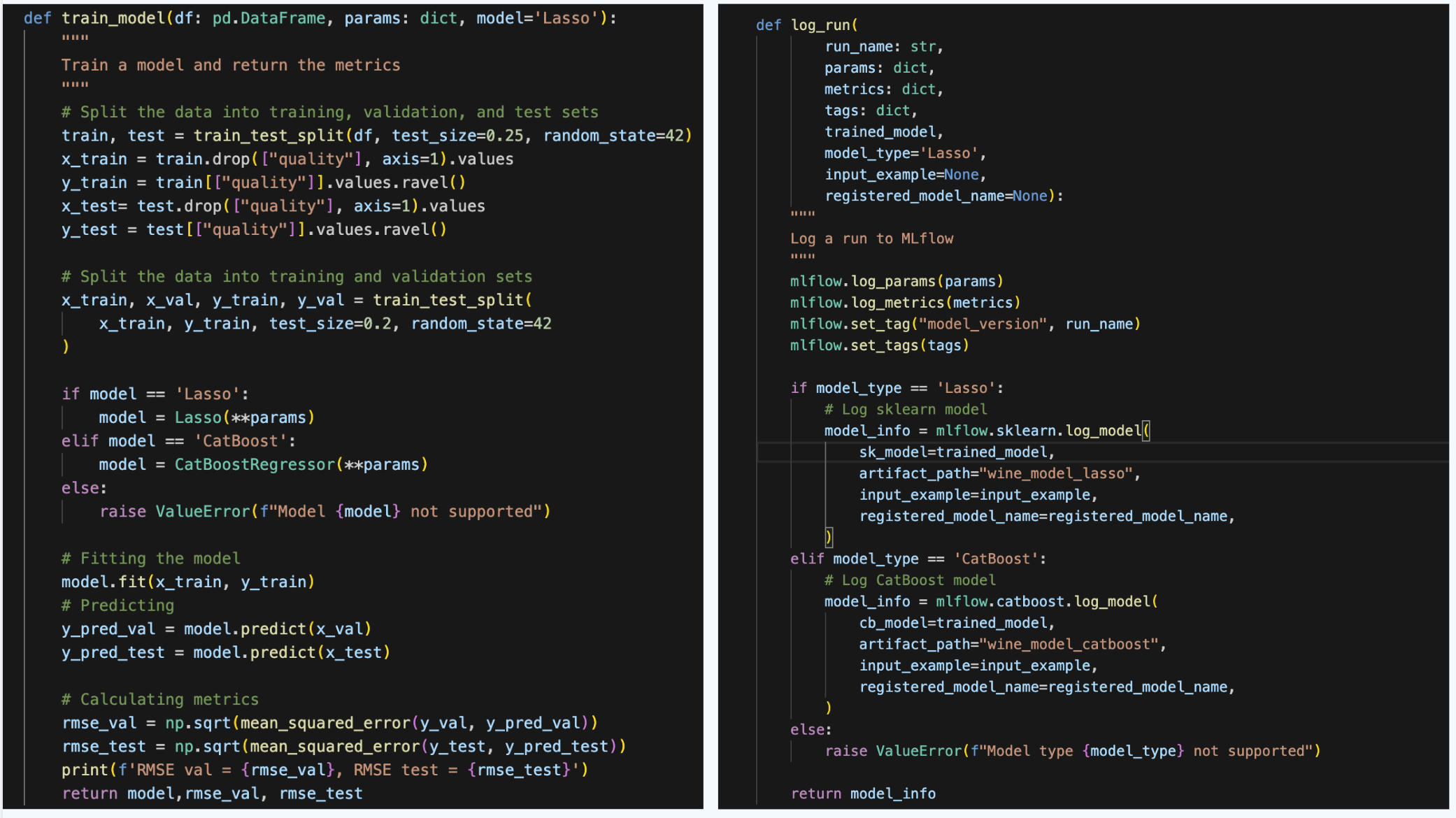
Running MLflow experiments with different models

Now, let's make our code a bit more modular, so we can efficiently run experiments for different models without code repetition. We make 2 functions: train_model and log_run.

Now, let's run the code for the LASSO model first, so we can start comparing the experiments for the same model type:

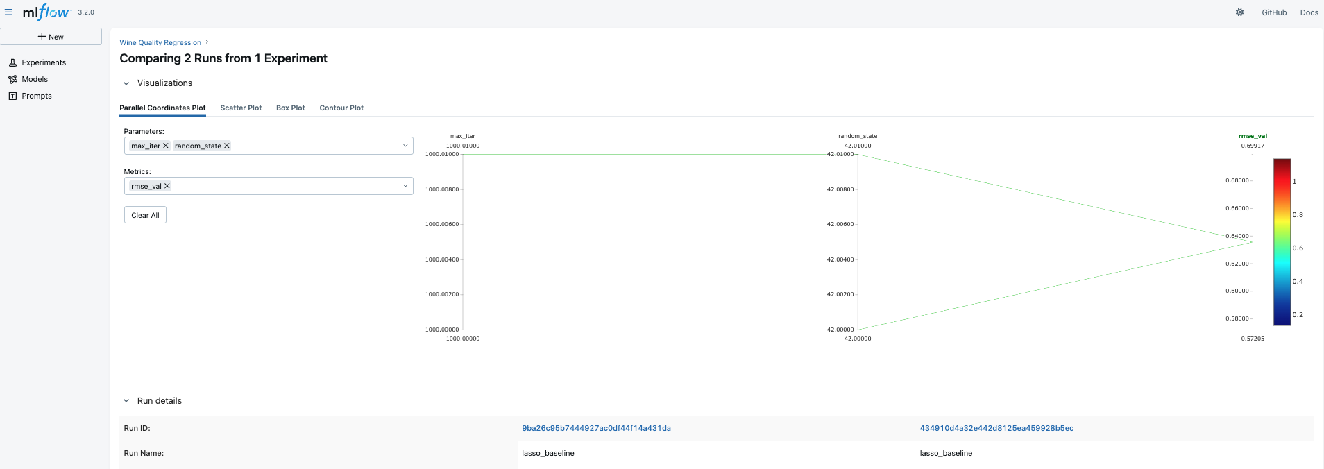
 We can then see that we created another run for the Wine Quality Regression Experiment. Now, we can select them and press Compare.

On the next page, we see the comparison of the RMSE metric. Since we have run everything with the same parameters, obviously, the results are the same. However, you can note that at the bottom of the figure, despite having the same run names and even the metrics, the Run IDs are different, so we can select a particular name based on this ID.

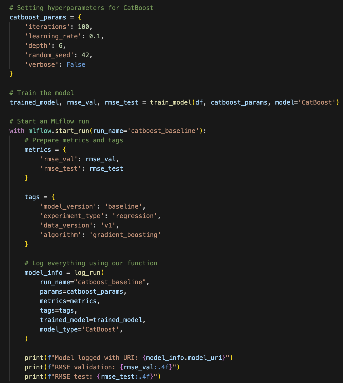
 Now, let's run and log an experiment with a CatBoost model.

Now, we can compare 3 different experimental runs - 2 LASSO and 1 CatBoost. To do that, select all the runs and press Compare as we have done above. Since the parameters are different for the models, the visual comparison of parameters might not tell much. However, we can compare the validation and test RMSE.

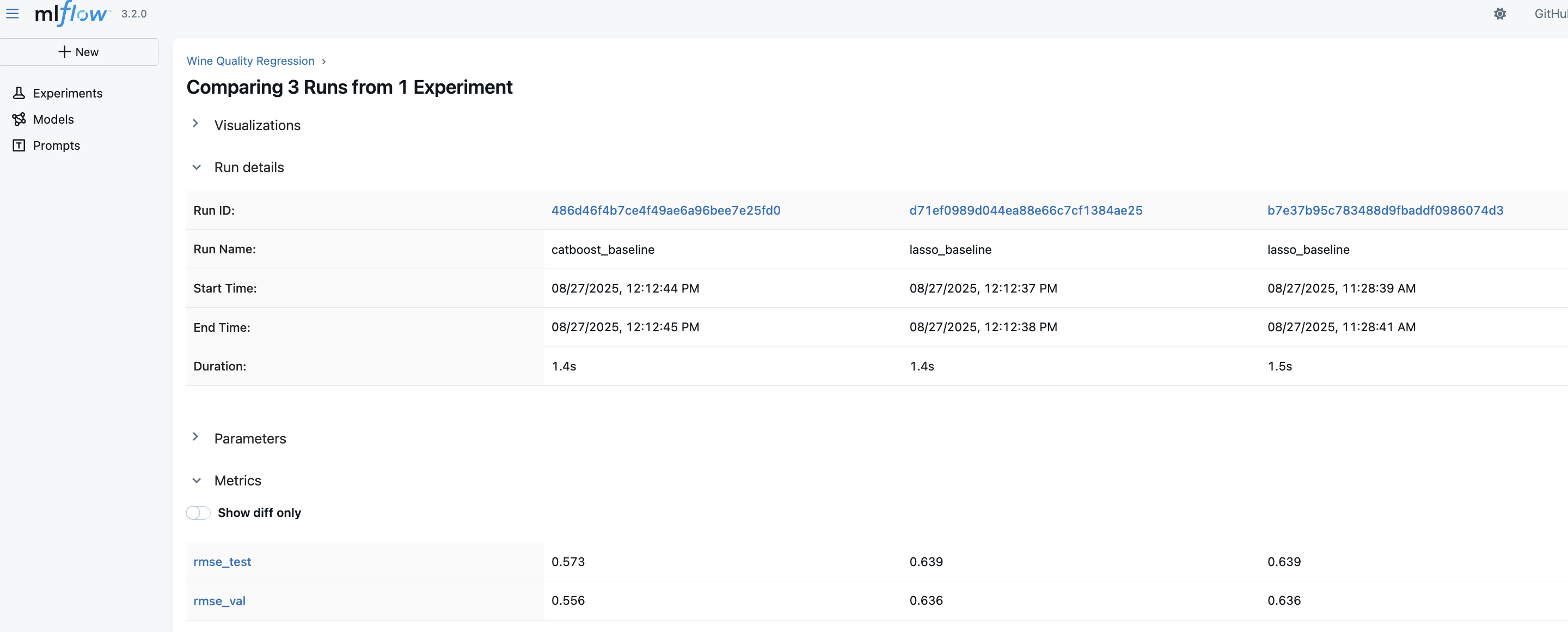
Here, we see that CatBoost outperformed LASSO, which is expected. But what is most important is that now you have a powerful tool to quickly compare the experiments and then select the best model to be deployed or to be taken for future experiments.

 

Finding the best model using MLFlowClient

Up to now, we could find the best model manually using the UI, which is great. However, when developing ML pipelines and registering the best model to be deployed, we need to be able to find this model programmatically. Here's how to do that.

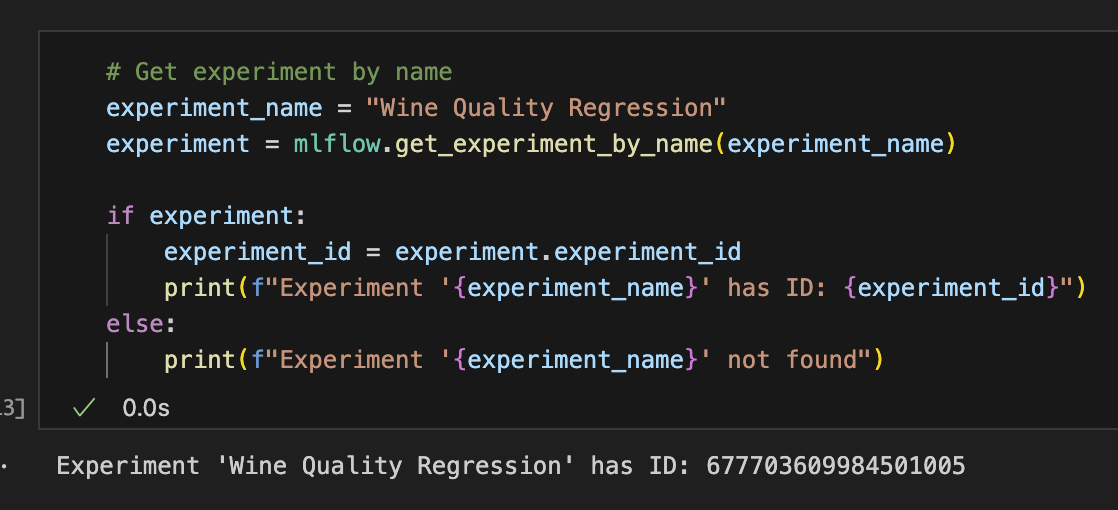
First, we need to find the experiment ID for which we want to select the best models. We can do that using search_experiments() method.

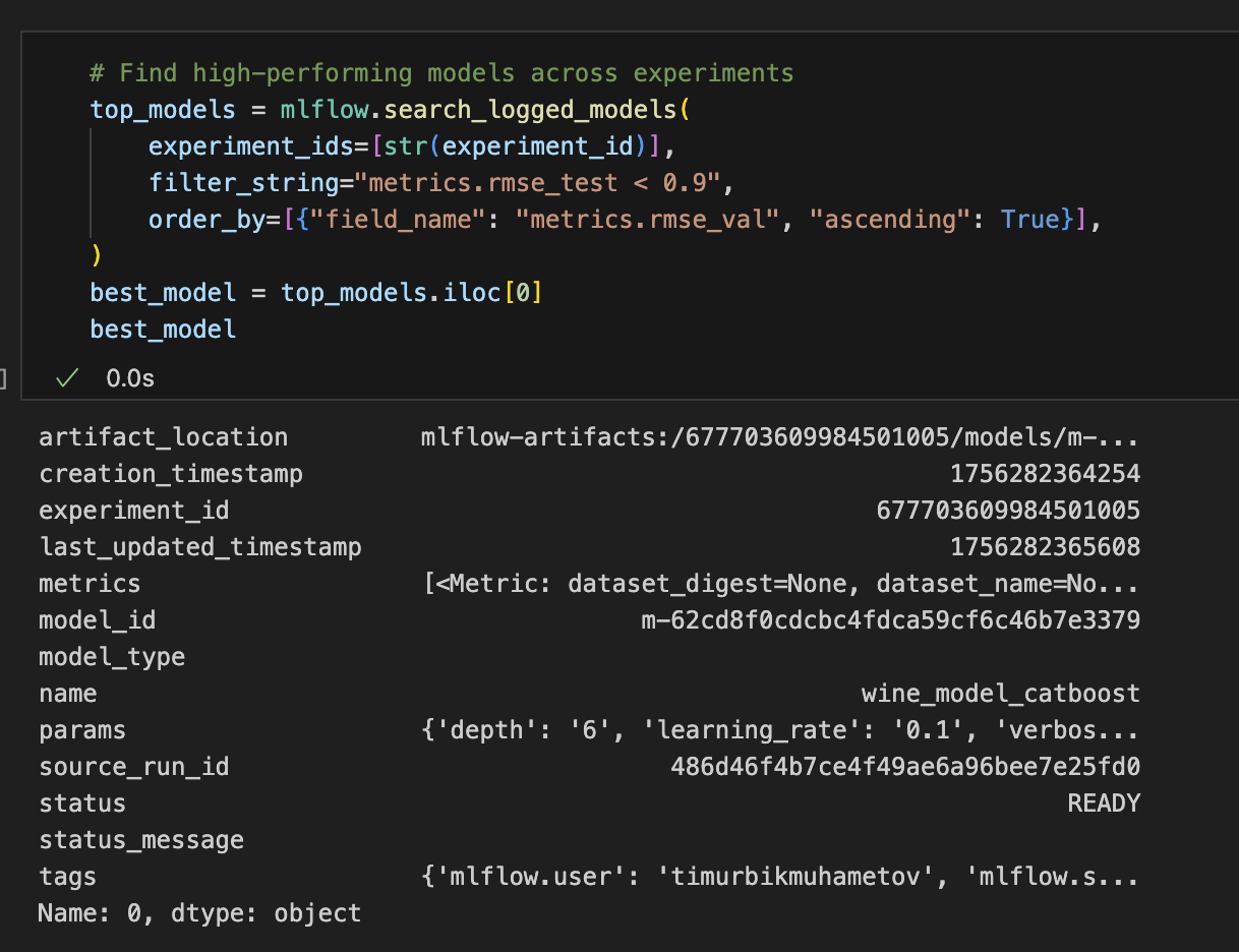
As we know the experiment ID, we can check what the top models are for this experiment and select the best model. To select the best model, we can just select the one at the top row of the resulting top_models dataframe. In our case, this is the CatBoost model.

Now that we have selected the best model, we can load it and make predictions.

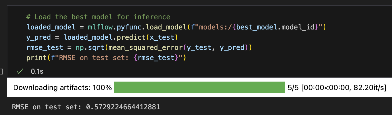
That's great! Now, we have a powerful tool to store and find the best models among any number of runs! Moreover, we can now use it in ML production pipelines because we can do this programmatically.

Recap

Ok, let's recap what we learned:

1. We know what is ML Experiment Tracking and why we need it

2. We know how to create an instance of MLflow Tracking Server and point to it using a URI.

3. We know how to create an experiment and ML runs.

4. We know how to log parameters for an ML run and compare parameters and performance between the runs.

5. We know how to programmatically load the best model among all the runs within an experiment and use this model to make predictions.

This basic MLflow functionality already allows us to do a lot of things.

However, there is some more functionality that can be useful. This will be covered in the next part of this tutorial.