Bayesian Optimization Introduction

If you've ever tried to tune hyperparameters for your ML models, you know how painful it can be. You basically have two options: either try a bunch of random values and hope for the best, or systematically test every possible combination using grid search.

Both approaches work, but they have one major problem - they're incredibly inefficient. You end up training your model dozens or even hundreds of times, and most of those training runs are a complete waste of time and computational resources.

But what if there was a smarter way? What if instead of blindly trying random hyperparameter values, we could actually learn from our previous attempts and intelligently decide which values to try next? That's exactly what Bayesian Optimization does. It treats hyperparameter tuning as an optimization problem and uses probabilistic models to figure out which hyperparameters are most likely to give us better results.

In this article, we'll dive deep into how Bayesian Optimization works, and I'll show you why it's so much more efficient than traditional methods like grid search and random search.

Bayesian Optimization of Hyperparameters. Problem Statement.

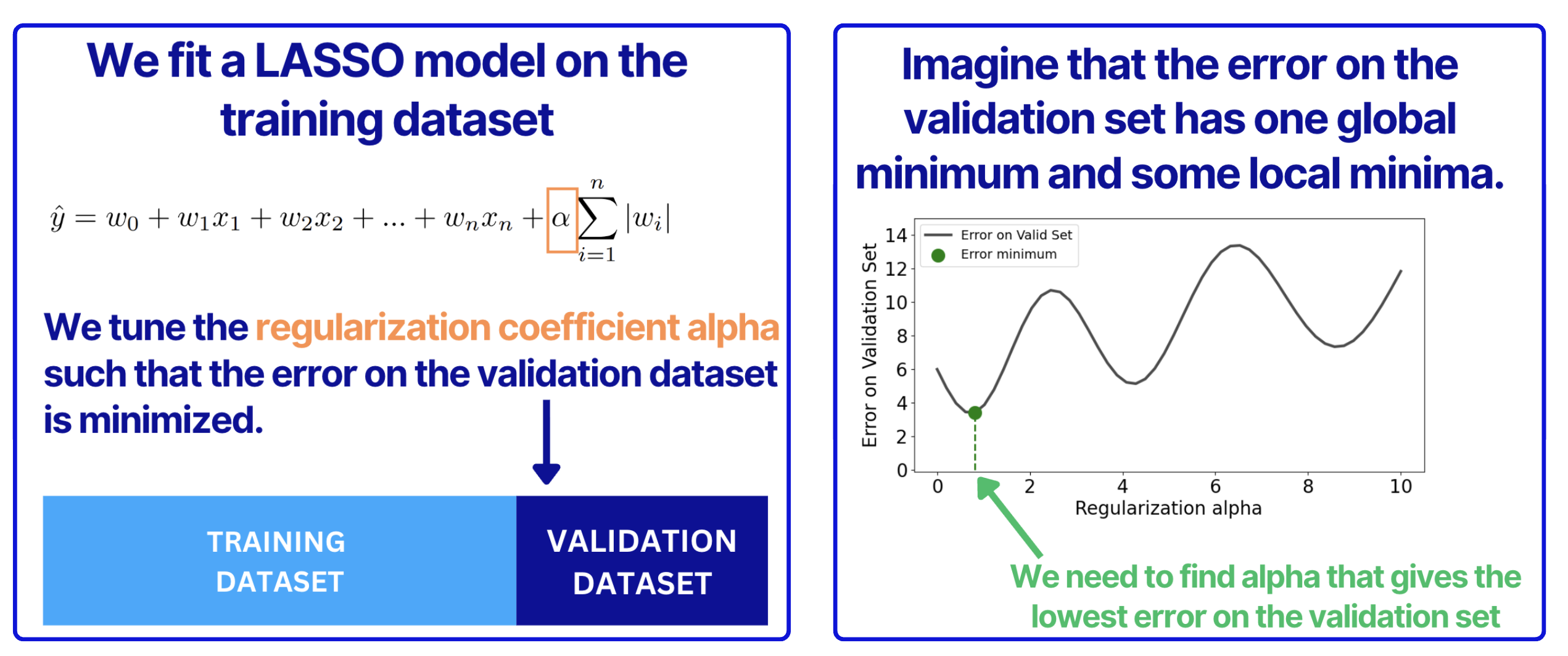
In this article, we will use the simplest possible example of hyperparameter tuning. We will tune a regularization alpha coefficient in a LASSO linear regression model. The way we are going to tune it is that we will try to find such an alpha that minimizes the error on the validation set.

So, for any given alpha and the model weights values, we can compute predictions and the error on the validation set. Now, let's imagine that the error on the validation set has not one but several minima. However, it has one global minimum that we ideally want to find. Finding this global minimum means that we found the best possible alpha given for these particular training and validation sets. As a result, we can expect good model performance on the unseen data.

Bayesian Optimization Algorithm

The main idea behind Bayesian Optimization is to create a model that predicts the error surface values (in one case, it's a 1D surface, essentially a grey curve in the figure above). In this case, we can just make predictions for any alpha value and take the minimum value among these predictions. But as for any ML model, we need a dataset. Let's make one!

Assume that we randomly selected 4 alphas and then for each alpha, we computed predictions and the error on the validation set, as shown below. 

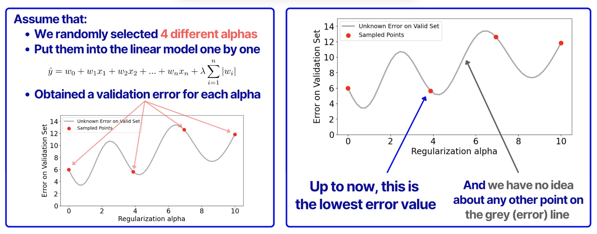
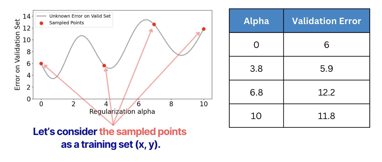
Then, based on these computations, we can find the lowest alpha that we can now. Also, we can then create a dataset to build a model that can estimate alphas for the rest of the curve (grey line).

Bayesian Optimization is called Bayesian because the ML models that are built based on the sampled points are probabilistic. This means that these models can estimate not only the most probable (Maximum Likelihood) values, but also the uncertainty of these predictions. As we will see later in the article, these uncertainties are used to understand which sample point (in this case, alpha) to try in order to minimize the objective function (in our case, it's validation set error).

There are two main Bayesian models that we used in Bayesian Optimization:

1. Tree-structured Parzen Estimator (TPE)

2. Gaussian Processes (GP)

In most cases, the current practice is to use TPE as it is usually more efficient to compute than GP, as well as natively support continuous and discrete variables. However, in this tutorial, we will use Gaussian Processes because they are easier to demonstrate. The overall idea will still hold for TPE.

Ok, let's get back to our problem.

So, we use the dataset to fit a Gaussian Processes model and estimate the most probable values of the validation set error and the uncertainty of the values. You can see the result of the modeling below.

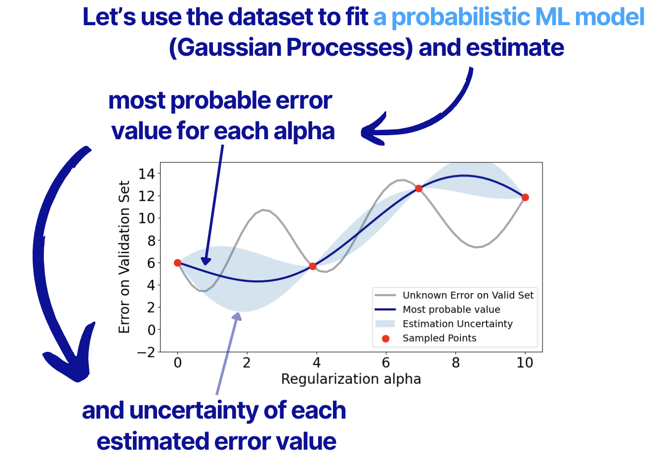
So, here's what we have up to now:

1. The minimum value of the validation error that we tested

2. Estimated most probable error values for all alphas.

3. Estimated uncertainties for these errors

Now, we can think of a way of using this info on how we can find the ACTUAL minimum error value.

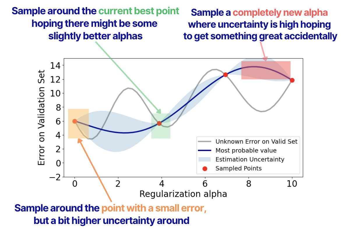
To do that, we have 3 strategies:

1. Sample around the current best point, hoping there might be some slightly better alphas

2. Sample around the point with a small error, but a bit higher uncertainty around.

3. Sample a completely new alpha where uncertainty is high, hoping to get something great accidentally

This is how these strategies can be visualized.

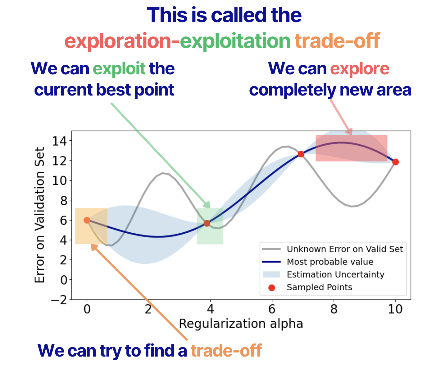
The selection problem between these strategies is called the exploration-exploitation trade-off. It essentially means that we can exploit the current best point and take samples just around the point we know for sure. We can also explore completely new areas. And finally, we can try to find a trade-off between these 2 strategies.

Now, as we understand the general approach, we need to define how we can use this strategy mathematically to search for the best alpha.

In practice, we use a so-called Activation Function. The Activation Function is essentially a mathematical formula that helps us decide which alpha to try next by balancing exploration and exploitation. It takes the estimated error values and uncertainties from our Gaussian Process model and outputs a score for each possible alpha - the alpha with the best score is the one we should sample next.

There are 3 most common activation functions:

1. Expected Improvement (EI) - This is one of the most widely used acquisition functions. It calculates how much improvement we can expect from sampling a new point compared to the current best result.

2. Probability of Improvement (PI) - This function measures the probability that a candidate point will improve upon the current best value. 

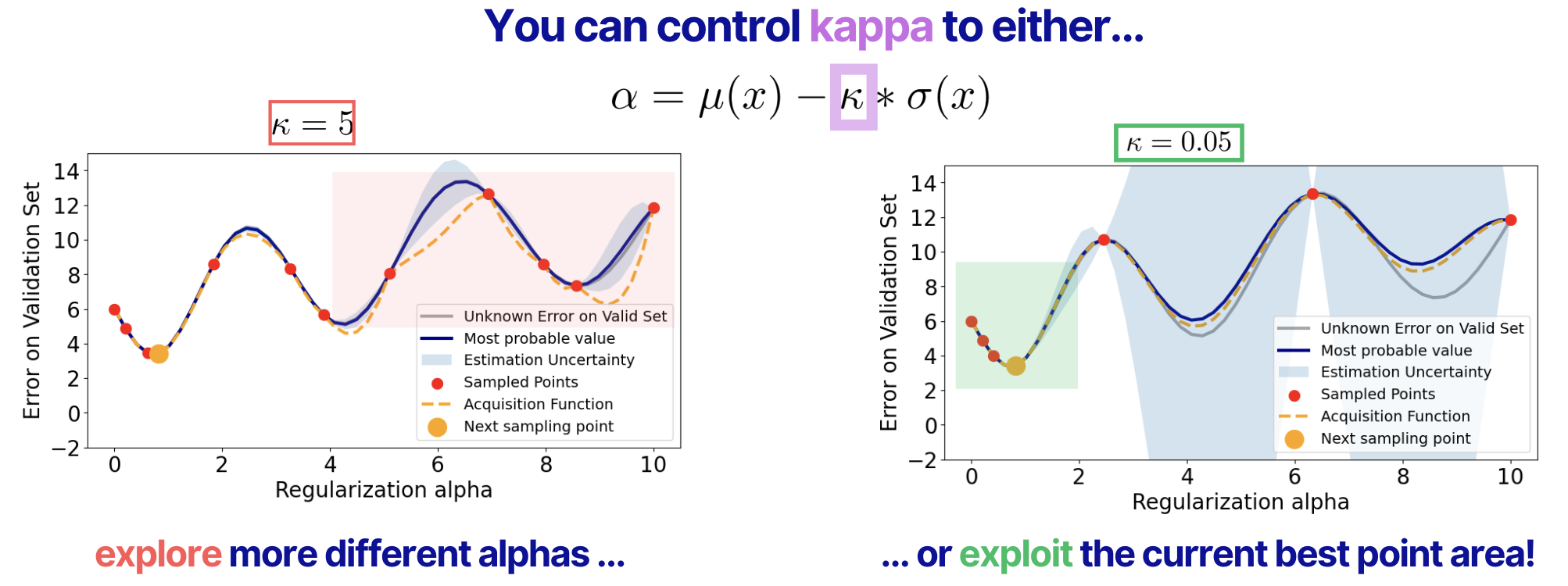
3. Upper Confidence Bound (UCB) (also called Lower Confidence Bound when minimizing) - This function balances the predicted mean with the uncertainty, using a multiplier to control the trade-off between exploitation and exploration. 

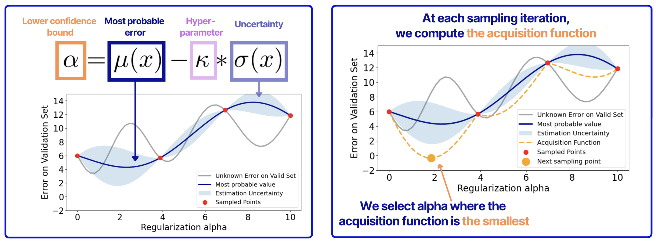
In our example, we will use Lower Confidence Bound (LCB), which is a minimizing version of the Upper Confidence Bound. Below, you see what the LCB looks like and how it works.

For each value of alpha (x in the equation), we compute the value of the LCB function. Then, to sample the next point, we find the smallest value of the LCB function, take the value of alpha, fit the model, make predictions on the validation set, and compute the validation error.

We are free to take as many samples as we want. However, remember that for each sample of alpha, we need to retrain the model and then compute the validation error value. In this example, we use a LASSO model, so the model training is nearly instantaneous. But if your model training is costly, the number of samples you can take is limited. And this is exactly where Bayesian Optimization helps - it allows you to find good hyperparameter values (i.e., the ones that give the minimum validation error) within a limited number of samples!

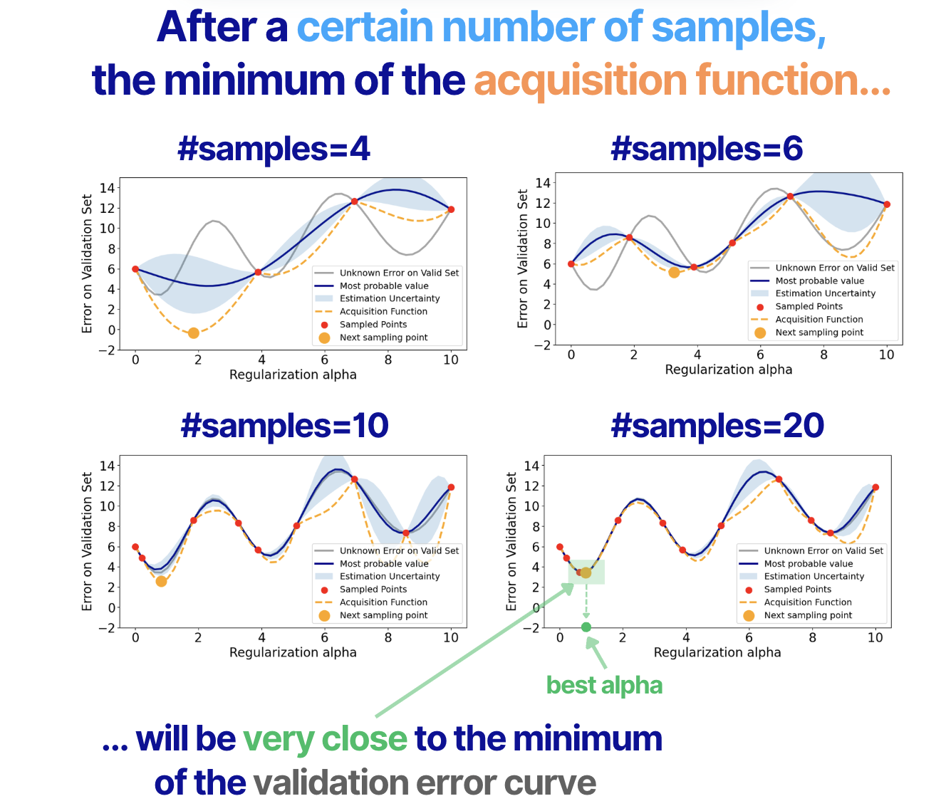
 Now, let's see how it works in our example. In the figure below, we see that as the number of samples grows, we get closer and closer to the global optimum of our validation error function.

As another quick example, you can see how this works in motion.

There is another important point to discuss here. In the formula of the LCB acquisition function, we have the parameter Kappa that we can use to give more priority to the exploration of the new areas or to the exploitation of the current best sampled point. In the figure below, you see that we Kappa=5, we tend to explore more (many points in the red box) or we can exploit more (most of the points are around the current best sample).

Bayesian Optimization vs Grid Search vs Random Search

Now, when we know how Bayesian Optimization works, we can check out how it compares with "traditional" hyperparameter tuning methods - grid and random searches. Maybe we really don't have to bother and just use what we used in the good old days.

Here's an abstract example of a model validation error function as a function of two hyperparameters. At the figure's bottom, we see the taken samples. At the top, we see the objective function value for each sample, and in the middle, we see the cumulative value of the objective function as the number of samples increases.

In this example, we can clearly see how Bayesian Optimization takes better samples (with lower objective function values). This is especially clear in the cumulative objective function curve. In the bottom plot we also see that it has more samples around the global minimum.

How does it help?

Well, as we discussed above in the article, Bayesian Optimization really helps when model training and evaluation are costly. Because for the vast majority of cases, it converges to reasonable hyperparameter values quicker than traditional methods, which means it requires less training and evaluation trials.

Conclusion

So, that's Bayesian Optimization in a nutshell. The main idea is pretty straightforward - instead of randomly trying different hyperparameter values or exhaustively testing all possible combinations, we build a probabilistic model that helps us make smart decisions about which values to try next. This model estimates not only the most likely validation error for each hyperparameter value, but also the uncertainty of these estimates.

Then, we use acquisition functions like Expected Improvement, Probability of Improvement, or Lower Confidence Bound to balance between exploiting what we already know works well and exploring new areas that might give us even better results.

The real power of Bayesian Optimization becomes obvious when model training is expensive. Whether you're training deep neural networks, large ensemble models, or any other computationally costly models, Bayesian Optimization can help you find good hyperparameters much faster than traditional methods. Instead of wasting time and resources on hundreds of training runs, you can converge to reasonable hyperparameter values in just a fraction of the samples.

Of course, Bayesian Optimization isn't a silver bullet - it has its own computational overhead from building the Gaussian Process or TPE models. But in most practical scenarios, especially when your model training takes more than a few seconds, the benefits far outweigh the costs.

So next time you're tuning hyperparameters, give Bayesian Optimization a try - your GPU (not to mention CPU) will thank you!