ML Ranking Systems – Complete Introduction with e-Commerce Example

Building a ranking system for an e-commerce search engine is one of the most challenging, yet rewarding, Machine Learning engineering projects. It combines data ingestion and storage, data engineering, real-time processing, model training, retrieval systems, data streaming, personalization, and constant iteration.

In the previous article, we learned about the fundamentals of Search Ranking Systems, and how Machine Learning is incorporated into such engines.

In this article, we’ll walk through how to design a modern, real-world Machine Learning system for e-commerce search ranking.

We will cover the overall design process and architecture, data, features and modeling fundamentals (no code yet,  that will come in the next articles, so keep an eye for them!).

By the end, you’ll understand what real companies like Amazon, Etsy, Walmart, eBay, and Zalando actually build under the hood:

from data to features → from labels to training → from retrieval to ranking → from online serving to continuous improvement.

Let’s begin.

1. Why e-commerce Search Ranking matters

When a user searches for “running shoes” on an e-commerce website, they might see hundreds or thousands of products. But the user will most likely click something in the top 2–5 results, and they almost never go to page 10.

That means the ranking model directly decides:

• what products get viewed
• what products get clicks
• what products get purchased
• total revenue for the company

Ranking is the revenue engine of the business.

But don’t think of it like just sorting by keyword match. In a modern system, you must combine:

• textual relevance
• product popularity
• personalization
• user behavior
• availability & shipping times
• product embeddings and semantic similarity
• multi-stage ML algorithms

This is where system design matters.

This article will guide you through designing a production-ready ML ranking system for product search, starting from the moment a user types a query to the moment they see ranked results.

2. The real-world scenario: Product Search

We’ll use a realistic example:

User query: “running shoes nike”

Goal: Return the best possible list of products, ranked by predicted relevance and purchase likelihood.

Why did we select product search as an example of such a system?

Because it includes everything:

text processing, semantic matching, ranking models, behavioral signals, personalization, extremely low latency requirements.

Designing this system is an excellent introduction to ML ranking at scale. You will see how many things are happening simultaneously when you type such a simple query in your search engine.

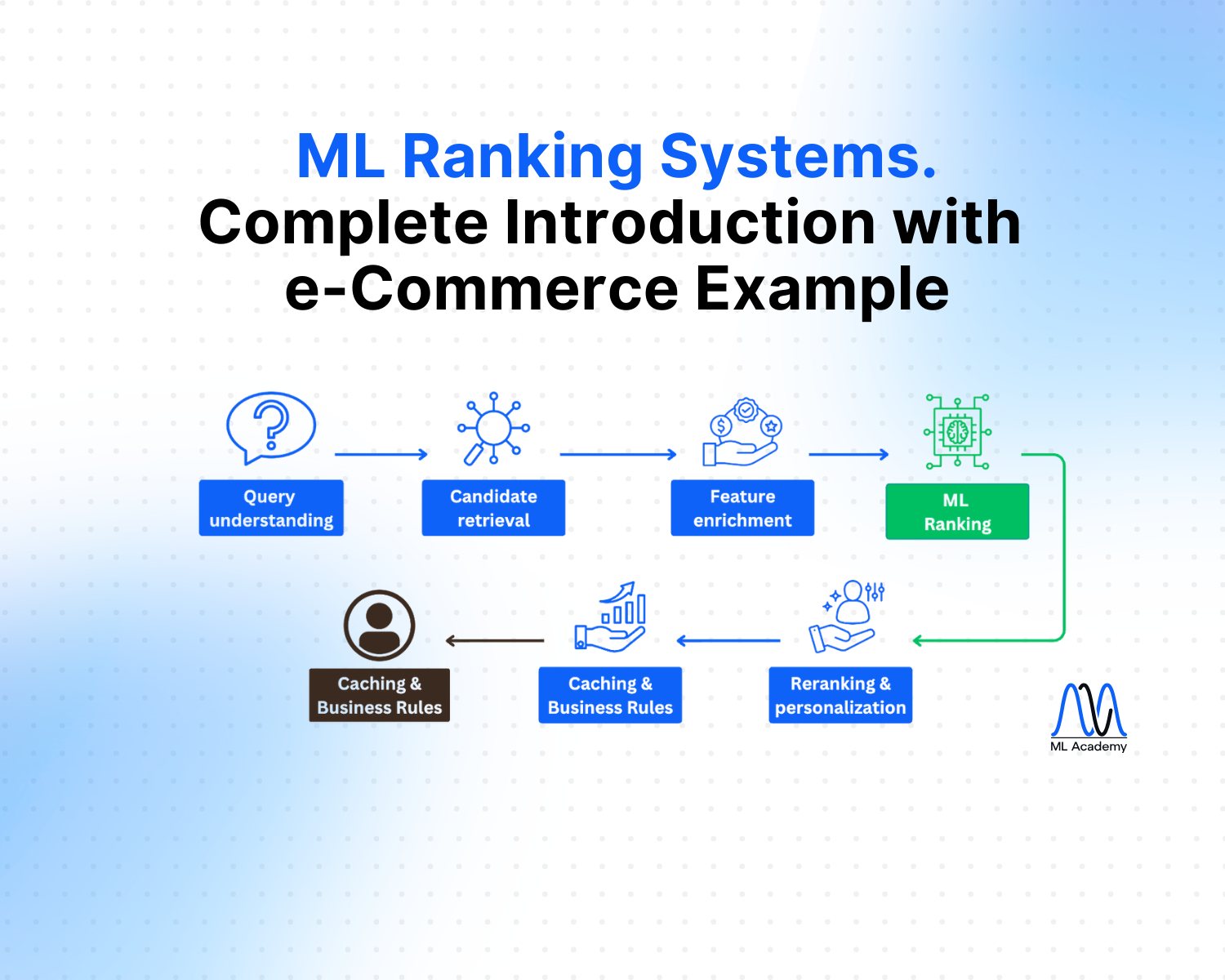
3. High-level architecture: How a modern ML Ranking System works

A modern search engine is always multi-stage. Instead of ranking all products, the system is designed to follow some steps:

1. Query Understanding & Processing
2. Candidate Retrieval (semantic & keyword-based)
3. Feature Enrichment (real-time feature fetch)
4. ML Ranking (LTR model)
5. Reranking & Personalization
6. Caching & Business Rules
7. Final Results

The above image represents the High-Level Architecture of an e-commerce Search Ranking System, in order to understand it conceptually first.

For now, let’s focus on understanding what is an ML Ranking System, the problem, the intuition and the overall components.

In the next article, we will view it in more detail and explain how everything is tied together.

We’ll keep this high-level mental image in mind as we dig into data, features, labels and training.

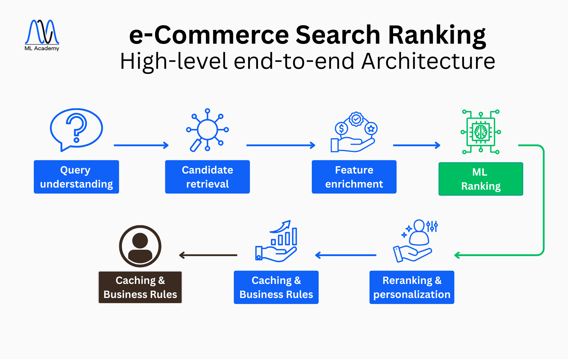
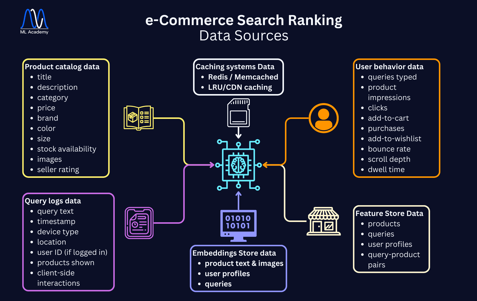
4. Data Sources: What feeds the Ranking System

A ranking system needs good quality data. And a lot of it.

In real-world e-commerce, there are several key data sources that feed the ranking model. In this introductory article, we’ll keep them conceptual, without diving into storage and infrastructure; we’ll do that in the next article, which will be about the overall ML System Design.

Think again about the query “running shoes nike”.

So what are all the Data Sources about? Let’s summarize with the help of this image:

‍

4.1 Product Catalog Data

This group of data is about product characteristics, such as title, description, category, price, brand, color and size. Think of it like, “what would characterize a pair of running shoes?”

Also, stock availability, images and seller rating belong to this category, as they define the stores that are going to be presented to you.

All the above data tells the system what each item is (and how it’s described to users).

4.2 User Behavior Logs

This type of data is derived from clickstream tracking (what are the user’s actions when viewing the results) and is mainly around queries typed, product impressions, clicks, and purchases.

Also, user actions such as “add-to-cart”, “add-to-wishlist”,  or time-related information like bounce rate, scroll depth, and dwell time (how long they stay on a product page) are considered to belong in this group of data.

Such logs are a great source of information because the system “understands” what the user possibly likes or not, based on the clicks, the interests (with add-to-cart or wishlist) and the viewing time. However, it is important to remember that, apart from “purchases”, everything else should be considered as “user intentions” or “user preferences” rather than “user reality”.

4.3 Query Logs

This is additional data about the user’s search queries, that could provide time-related and geographical information. 

Each search query is logged with query text, timestamp, device type, location, and user ID (if logged in). Additionally, products shown and client-side interactions can provide meaningful information.

Considering the above, we see that query logs help with understanding intent, building query embeddings, and finding popular queries so that we can generating training data for our ranking models.

4.4 Embeddings Store (Conceptual View)

An Embeddings Store is a specialized database designed to store vector representations of items, queries, users, or even images. 

In our example, a vector representation of “running shoes” is a numerical embedding that captures its meaning, placing it close in space to related concepts like “sneakers” and far from unrelated ones like “office chair.”

To better understand it, a vector representation of “running shoes” could be this array of numbers: [0.12,  -0.48,  0.91,  0.07,  0.33,  -0.22,   0.56,  0.14, -0.37,  0.80].

Such vectors can be constructed by language models, which can convert a word into a high-dimensional numerical representation that captures its semantic meaning. Different training datasets can create different vectors for the same words. Now, if you also calculate a vector for “sneakers” and compute their cosine similarity, you will find out they are close enough to be considered both as “shoes”.

Going back to the Embeddings Store, think of it like a database but, instead of traditionally storing text or numbers, it stores high-dimensional vectors (e.g., 256-dimensional or 768-dimensional) like the example above, that encode meaning learned from neural models.

But why does it matter in our use case?

When ranking products in e-commerce, simple text matching (“running” matches “running”) is not enough. Embeddings allow the system to understand semantic relationships:

• “running shoes” ≈ “fashion sneakers”
• “sofa” ≈ “couch”
• “formal wear” ≈ “dress shirt”

This enables better retrieval, better ranking, and more personalization.

We’ll dive into where and how these embeddings are stored and searched in the System Design article.

4.5 Feature Store (Conceptual View)

A Feature Store is a system that stores, manages, and serves machine learning features consistently for both offline training and real-time inference.

It solves one of the biggest problems in ML systems, that the model doesn’t see the same features in training and in production.

It actually does that by providing:

1. Consistent features: the same code produces the same feature values during both training and inference processes.
2. Low-latency online access: the ranking model needs hundreds of features within milliseconds.
3. Feature versioning: if a feature changes (e.g., new definition), older models can still use the old version.
4. Historical feature lookup: needed to create training data with features as they existed at that time.

In this introduction, it’s enough to remember:

Feature Store = “single source of truth” for ML features, used both offline (for training) and online (for live ranking).

4.6 Caching Systems

Now imagine you search for these “running shoes nike” and you wait even for 10 seconds. You will refresh the page or leave entirely, right?

That;s why Caching is essential, because ranking systems must answer queries fast, usually under 100–200 milliseconds end-to-end. Without caching, the system would have to repeatedly compute expensive features, run complex retrieval logic, or fetch data from slower databases.

Caching helps by storing:

• frequent query results (e.g. “iphone case”, “black dress”)
• commonly used features
• precomputed pieces of logic

5. Feature Engineering: The Heart of the Ranking Model

A ranking model does not take a single vector of a couple of features. It considers multiple feature groups, with often hundreds of features.

Let’s break them down.

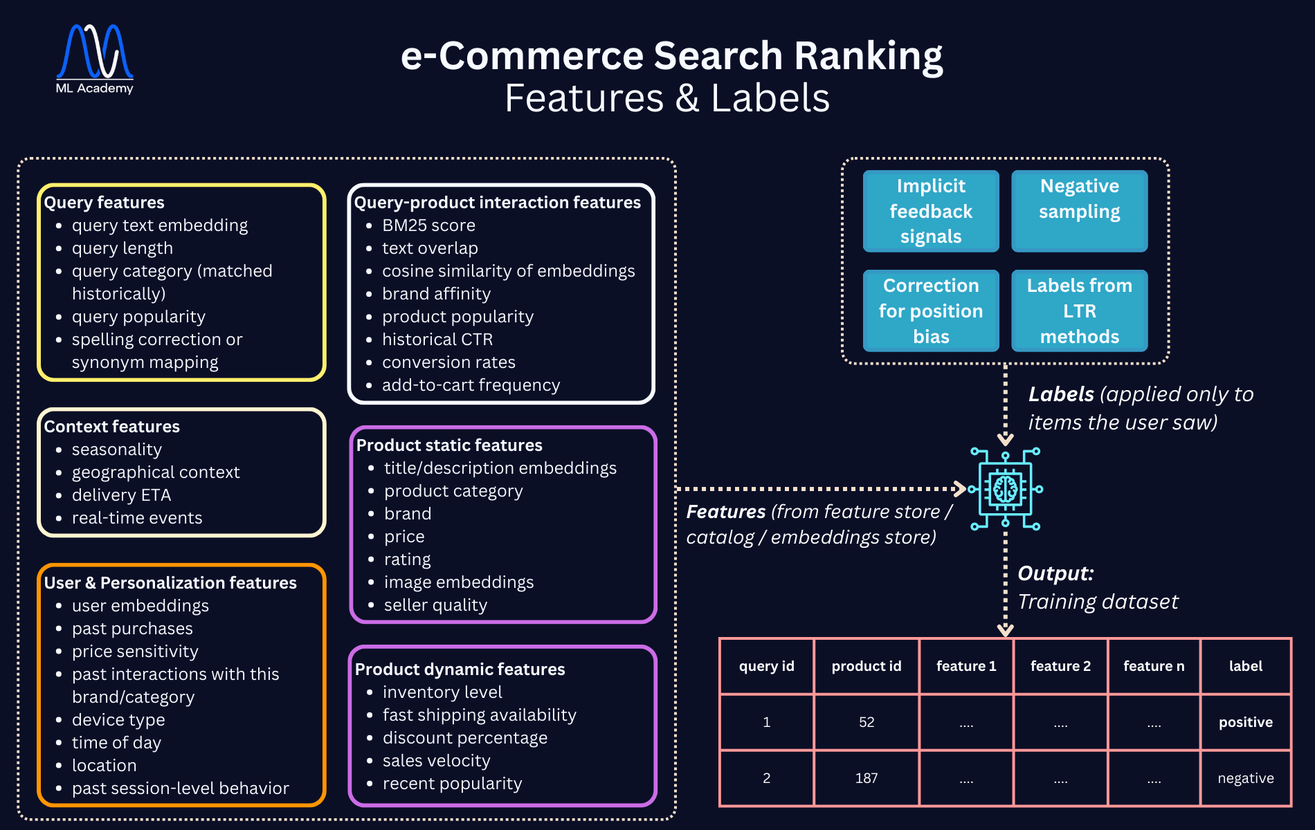
5.1 Query Features

Query features describe the search query itself, what the user typed and how the system interprets it.

Different queries imply different intent, for example “running shoes men” is different from “nike zoomfly review”, even if they both involve shoes. The model needs signals that help capture this nuance.

Some indicative features involve query text embeddings, query length, query category (matched historically), query popularity, and spelling correction or synonym mapping.

These features help the ranking system understand what the user is looking for, even before considering any products.

5.2 Product Features

These ones describe the individual items in the catalog. They help the model understand what each product is, regardless of who is searching. We have two sub-categories:

• Static features (don’t change often):
  
  • title/description embeddings
  • product category
  • brand
  • price
  • rating
  • image embeddings
  • seller quality
• Dynamic features (change frequently):
  
  • inventory level
  • fast shipping availability
  • discount percentage
  • sales velocity
  • recent popularity  

Product features ensure that the model knows what kind of item it is ranking and whether it’s appealing from a business/quality standpoint.

These are the most important features in ranking, as they describe the relationship between a particular query and a particular product:

• BM25 score: a classic search relevance score (we talked about it in the previous article)
• text overlap: how many words from the query appear in the title/description
• cosine similarity of embeddings: match “camper shoes” with “running sneakers”
• brand affinity: does the user like Nike?
• product popularity: for this query
• historical CTR: for this query-product pair
• conversion rates: if users often buy the product after that search
• add-to-cart frequency: stronger than click, weaker than purchase

Interaction features teach the model which product best satisfies this specific search, making them central to ranking quality.

They actually tell the model:

“For this specific query, how good is this specific product?”

5.4 User & Personalization Features

If the user is logged in, personalization features can significantly improve ranking, so the model can use user embeddings, past purchases, price sensitivity, and past interactions with this brand/category.

If not logged in or anonymous users, personalization still exists, but is now based on device type, time of day, location, and past session-level behavior. More generic features, but still important to reference the user.

Personalization ensures the ranking system feels tailored rather than generic (similar to recommendation systems).

5.5 Context Features

Such features help the ranking system react to the world around it, even when it lacks the previous feature categories, by considering:

• seasonality: winter jackets in winter or running shoes in summer)
• geographical context: some products sell better in certain regions (snow boots vs sandals)
• delivery ETA: Estimated Time of Arrival, very important during holiday season
• real-time events: Black Friday, sales, holidays

​​Context features make the system adaptive, avoiding the one-size-fits-all problem.

6. Label Generation: How the Model Learns What’s “Good”

Ranking models need labels to learn what “good search results” look like. Think of it like Supervised Learning, where you need labeled data to teach the algorithm how to make correct predictions.

But in e-commerce, labels are not simple, because we do not ask annotators to mark each document as “relevant.”

Instead, we use implicit feedback in different formats:

6.1 Implicit Feedback Signals

Every user action is linked with some sort of interpretation to better understand the intention and the likelihood of the action’s result.

‍

Let’s see how some indicative actions translate into feedback signals of purchasing:

• click → weak positive
• high dwell time → moderate positive
• add to cart → strong positive
• purchase → very strong positive
• skip result → likely negative
• low dwell time → weak negative

How do we interpret all of this?

“Clicks” is the simplest form of positive feedback. When you click an item, it suggests the product looked relevant to the query, and “high dwell time” shows how long you stayed on the product page. Longer dwell time usually indicates genuine interest, but “add-to-cart” actually indicates that the product was not only relevant but appealing.

What's more, “purchases” is the strongest implicit label, as it suggests the product perfectly matched your intent. However, purchases are sparse and must be used carefully to avoid “rewarding” popular products.

On the other hand, “skipping results” is useful negative information because it means that you saw the product but didn’t interact with it, while “low dwell time” ​​(1–2 seconds) is often a weak negative signal.

As you see, whatever action you make when searching something, gets recorded and gives feedback to the system as “labels”, to better understand your intentions.

6.2 Negative Sampling

Users see many products but interact with few (labeled as “positives”). But this doesn’t necessarily mean that all the rest products were not good; it might mean that the users didn’t scroll enough to find them. As such, they shouldn’t be labeled as “negatives” the same way.

So, for each query:

• clicked items → positive
• non-clicked items in top results → negative

What this means is that only products you actually saw (e.g., on the first page or first screen) and ignored should be marked as “negatives”. If a product was far down the list and never scrolled into view, it should not be labeled negative.

On the other hand, there are products that you frequently see but never click, and these should be labeled as “hard negatives”.

If there are too many negatives, the model may dominate on negative samples and stop learning positive relevance (class imbalance problem, very usual in ML), so the model should be designed to achieve balanced training, where it typically samples:

• a small subset of negatives per query
• or weight negatives lightly

This would prevent the model from falling into the “class imbalance” issue.

Here is an illustrative example of how Negative Sampling works, where the user sees 7 products (4 in the 1st search page and rest in the 2nd page), and what is finally labeled as “positive”, “negative” or “ignored”:

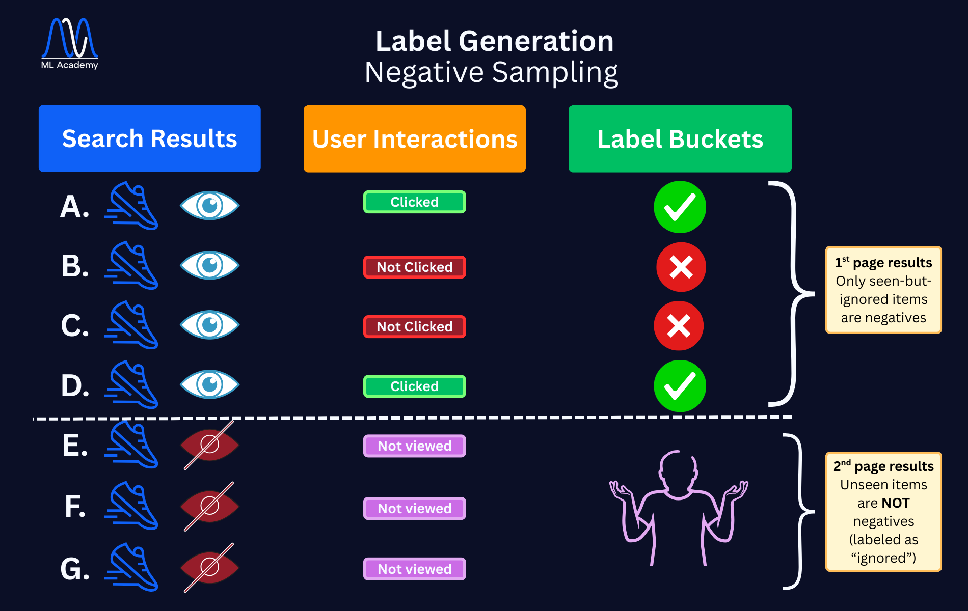
As seen in the image above, the items that the user viewed and clicked are labeled as “positive”. However, only those products seen but not clicked should be marked as “negatives”, and not everything else. Also repeatedly ignored (not clicked) items are marked as “hard negatives”.

Products that weren’t viewed at all should be simply marked as “ignored”, and the system can use sampling/weighting to avoid negative-label dominance.

6.3 Correcting for Position Bias

Users click higher results more because they’re higher, not necessarily because they’re better.

If we naïvely treat “clicked = good” and “not clicked = bad,” the model will incorrectly learn that whatever it previously ranked highly must be correct, creating a self-reinforcing loop.

Two solutions:

• Randomized experiments: swap positions temporarily, shuffle items for a tiny fraction of users or run interleaving experiments.
• Propensity scoring: each click is weighted inversely to the probability that an item was viewed because of its rank. For example, items at the top receive less weight because they get “easy clicks”, while items lower in the list receive more weight when clicked because you intentionally scrolled to them.

Without these corrections, the model will reinforce its own mistakes.

7. Training the Ranking Model

This is where ML begins (at last!)

Now that we have labeled data and a rich set of features, the next step is building the training pipeline for the ranking model. 

Unlike typical ML workflows, ranking requires careful preparation of query–product pairs, consistent offline/online features, and evaluation targeted specifically to ranking performance.

Let’s see how this combination of features and labels happen, and what the training set would look like:

7.1 What the Training Data Looks Like

At the end of the data pipeline, you usually get something like this:

query_id | product_id | feature_1 | feature_2 | … | feature_n | label

For example:

• query_id = 1 might correspond to “running shoes nike”
• query_id = 2 might correspond to “running shoes”

And label might be:

• 1 for positive
• 0 for negative

But in practice, there are more nuanced labels and ranking paradigms.

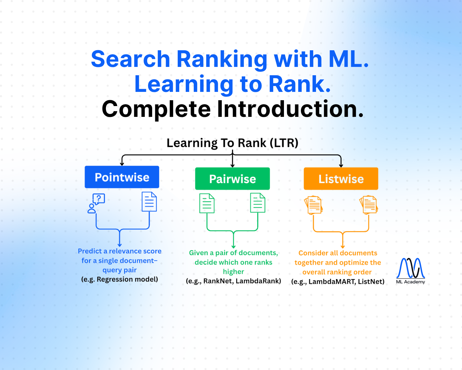
7.2 Learning to Rank (LTR) Paradigms

In the previous article, we talked about a special kind of Supervised Learning: Learning To Rank (LTR).

LTR models in this case are trained on historical data where queries, products and user interactions are known and each query–product pair is given a label indicating the relevancy.

The model then learns a scoring function f(q,p) that predicts how relevant a product p is to a query q.

When a new query arrives, it scores all candidates and sorts them by predicted relevance. The most usual methods are:

• Pointwise: These treat the ranking problem like a regression or classification task:
  
  • click = 1
  • add to cart = 2
  • purchase = 3
  • no interaction = 0

Pointwise is simple but doesn’t account for relative ordering of results, so it’s rarely used anymore.

• Pairwise: Pairwise models (like RankNet) learn that:

“For this query, product A should rank higher than product B.” These labels are built by comparing:

• clicked - unclicked items
• high dwell - low dwell
• purchase - skipped

Pairwise is stronger because ranking is fundamentally about ordering, not absolute scores.

• Listwise: Such methods (like LambdaMART or NDCG-based training) operate on the entire result list:
  
  • They learn patterns across all items shown together.
  • They optimize for metrics like NDCG, which directly rewards correct ordering near the top.

This method aligns best with real-world goals.

Most production systems use pairwise or listwise.

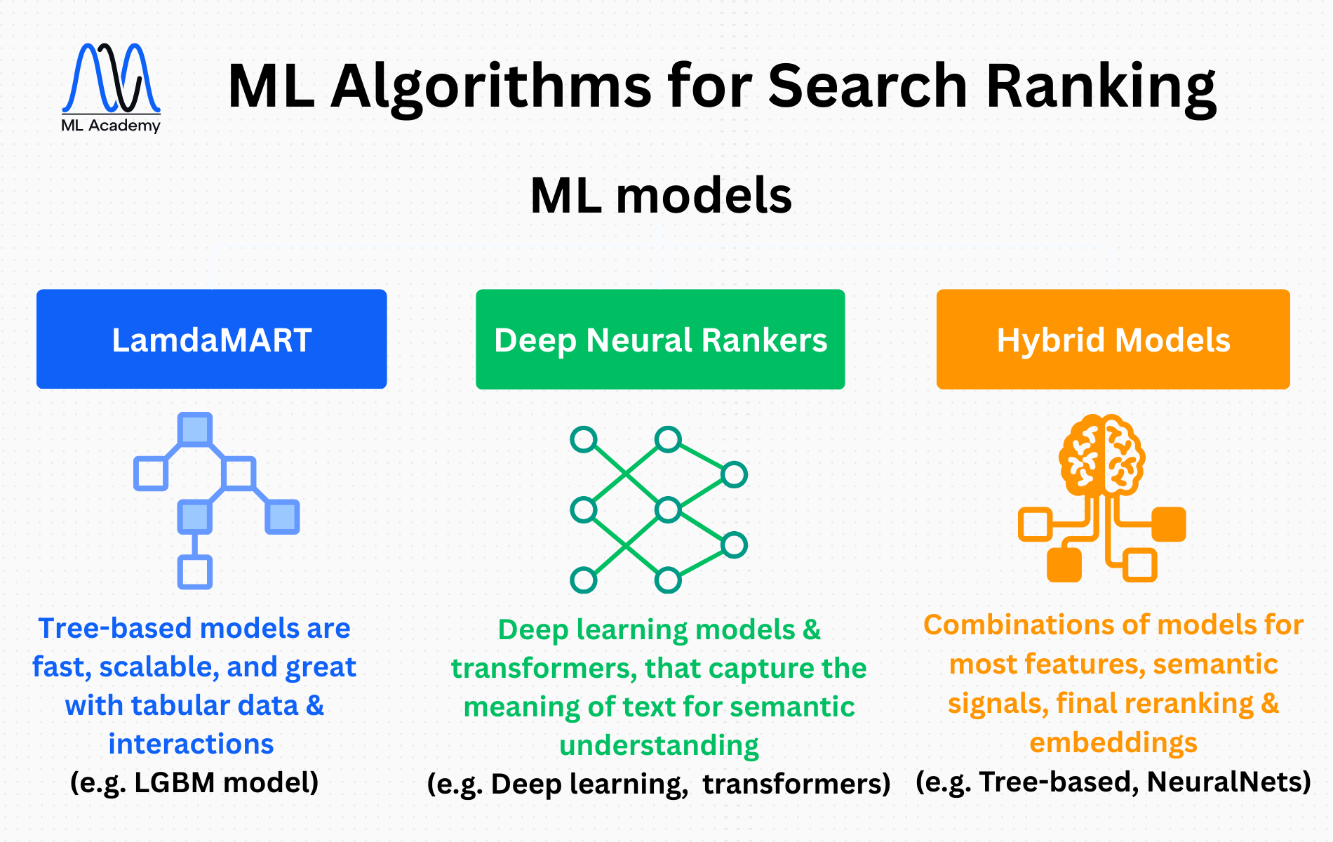
7.3 Algorithms Used in Practice

The three most common algorithms in industry:

7.3.1. LambdaMART (implemented in LightGBM)

Tree-based models dominate many real-world ranking systems because they are:

• fast
• scalable
• very strong baseline
• great with tabular data and interaction features
• used by many big companies (Bing, Yahoo search historically)

7.3.2. Deep Neural Rankers (Bi-Encoders, Cross-Encoders)

Deep learning models, especially transformer-based ones, that capture the meaning of text better than any manual features or BM25 scores and are known for:

• excellent semantic understanding
• fast inference
• very high accuracy
• high cost of running
• slow training (usually used for re-ranking top ~100 candidates)
• often layered on top of tree-based models for fine-grained improvements.

7.3.3. Hybrid models

The most modern production systems use a combination:

• Tree-based models for most features
• Neural models for semantic signals or final re-ranking
• Embedding similarity models for candidate retrieval

With this hybrid approach we can achieve balance between performance, speed and interpretability.

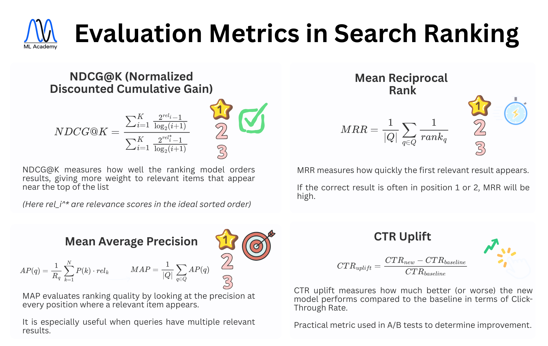
7.4 Evaluating Ranking Models

Ranking tasks use different metrics than classification, which means that accuracy, precision, recall and F1-score don’t make much sense here.

The main ones, instead, are:

• NDCG@K (Normalized Discounted Cumulative Gain): rewards correct ordering, especially near the top of the results
• MAP (Mean Average Precision): useful when queries typically have many relevant items
• MRR (Mean Reciprocal Rank): measures how quickly a model finds the first relevant result
• CTR uplift: used in offline evaluations as sanity checks, or in A/B testing

7.4 A/B Testing Stage

Even if offline metrics look good, nothing matters until:

• CTR improves
• add-to-cart improves
• revenue improves

The final judge is always A/B testing with real users. 

To ensure success, companies run controlled A/B experiments, where users are split into two groups (“control”, that sees the old model, and “treatment” that sees the new model). Then they track real engagement metrics such as CTR, add-to-cart rate, purchase conversion, revenue/user and user satisfaction metrics.

They then measure statistical significance and, if “treatment” outperforms “control” they roll out gradually to expand traffic. In general they follow the rule: “If it wins online, the model is good, otherwise you iterate again”.

8. What Happens at Query Time (Real-Time Ranking – Intuition)

Let’s go back to the real-time side and walk through what happens when a user types a query.

Imagine the user types:

“running shoes nike”

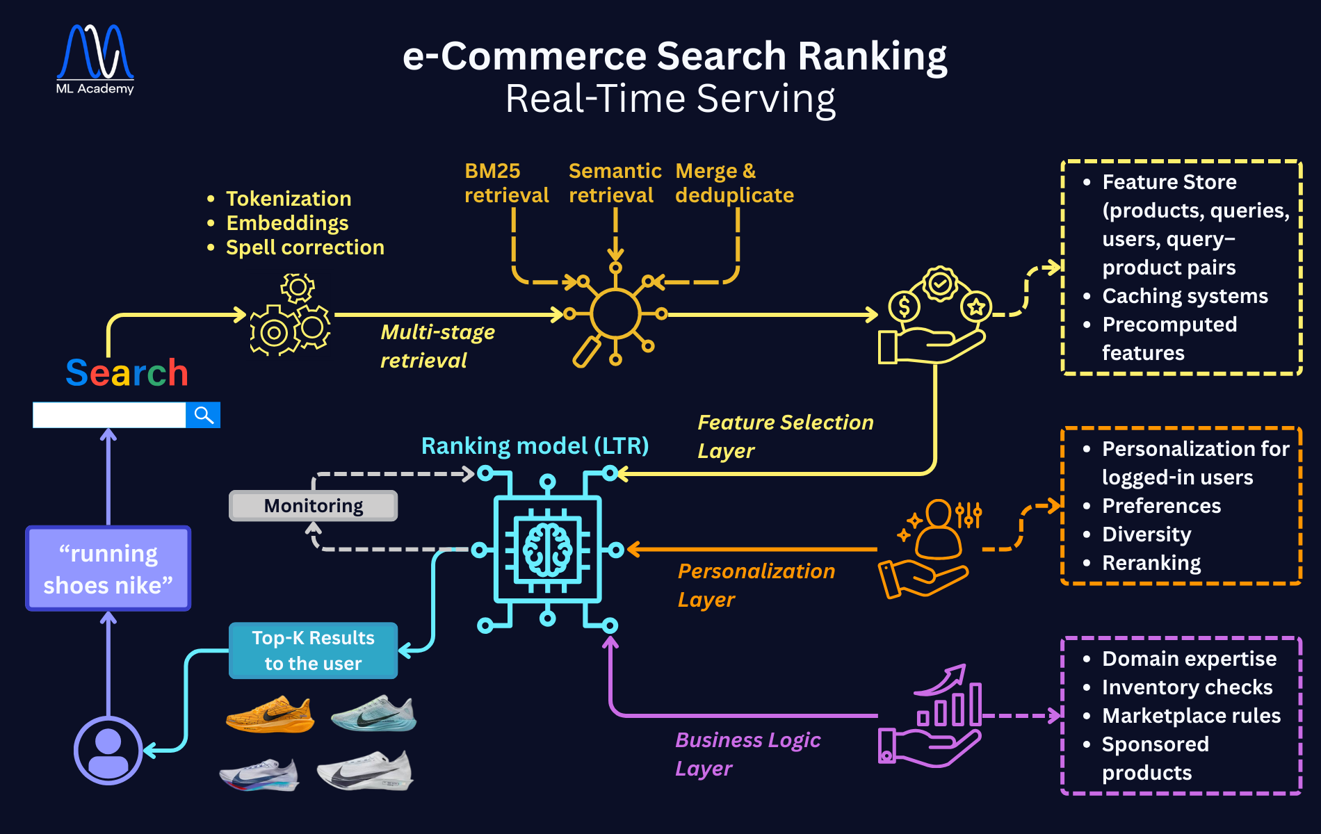
8.1 Query Processing

The pipeline begins the moment the user types a query. Query processing prepares the text so both retrieval and ranking can work effectively.

The system:

• tokenizes and normalizes the query
• fixes spelling where needed
• generates a query embedding (for semantic matching)
• optionally detects intent (brand search, category search, product review search etc.)

8.2 Multi-Stage Retrieval

Why multi-stage?

Because you cannot run a neural model on the whole catalog and operate in milliseconds.

Modern systems use two complementary retrieval paths:

1. BM25 Retrieval
   This retrieves products that contain query terms, such as title, description, category or attributes, and is simple, fast and returns top 500 candidates.
2. Semantic Retrieval
   This retrieves products whose meaning matches the query, even when the keywords differ, using vector similarity to find semantically similar items.

Returns another ~200 candidates.

Finally: Merge & Deduplicate
Combine the two sets (keyword + semantic) and remove duplicates.

So the final candidate set might usually be 200–1000 products.

Only these candidates are passed to the ranking model.

8.3 Feature Selection

This is the biggest engineering challenge because the ranking model needs hundreds of features per candidate.

For each candidate product, the system fetches information about query features, product features, interaction features, user features, and context features.

Feature Selection must happen extremely fast, sometimes within 5–20ms, so it requires an online Feature Store, caching and precomputed features.

8.4 Ranking Model Inference

The ranking model evaluates each candidate, forming a function like:

score = f(query_features, product_features, interaction_features, user_features)

The top results go forward.

This is often done by LightGBM with LambdaMART, XGBoost ranking or a simple neural model. We aim for high accuracy with very small latency and low cost.

Neural rankers, as we said before, might be applied only to top 50–100 results due to cost as second-level rankers.

8.5 Reranking & Personalization

After initial ranking, the system may apply personalization, especially for logged-in users, in order to push more relevant brands for this user and boost fast-shipping items. Additionally, it can avoid showing three nearly identical products in a row, while also diversifying category distribution.

For example:

• If user A buys premium running shoes, then boost high-end items.
• If user B buys budget shoes, then boost lower-priced items.

These business-focused layers make the experience feel “high quality.”

8.6 Final Layer: Business logic - Domain expertise

After ML is done, the final step is about compliance to business constraints. This is crucial because real-world e-commerce must follow rules outside machine learning.

Common logic, along with domain knowledge (it’s all around humans, after all), includes:

• Remove out-of-stock products
• Block restricted or banned items
• Boost sponsored/ad products
• Boost promoted brands during marketing campaigns
• Demote products with poor seller ratings
• Avoid duplicates (same product in different colors)

This ensures the final results are safe, compliant, profitable, and diverse.

9. Summary & What Is Next

Let’s quickly recap what you’ve learned in this introduction:

• Product search is one of the most ML-heavy problems in e-commerce.
• Modern search engines use multi-stage ranking: retrieval → ML ranking → reranking → personalization → business rules.
• The ranking model needs rich data from many sources: catalog, user logs, query logs, embeddings, feature stores.
• Features are mainly grouped into query, product, interaction, user, and context features.
• Labels come from implicit feedback signals like clicks, dwell time, add-to-cart and purchases, with care around negative sampling and position bias.
• Ranking is a Learning to Rank problem, often solved with LambdaMART, neural rankers, or hybrids.
• Real-time ranking involves: query processing, multi-stage retrieval, feature fetching, ML scoring, personalization, then business rules.

This article was about building a solid mental model for ML ranking systems, using e-commerce as a concrete example.

In the next article, we’ll go more in detail into the system design and architecture side:

• how these components are actually wired together
• how data pipelines are built
• how the feature store, embeddings store and caches work
• how monitoring, drift detection and continuous learning are implemented in production

So next time you search for “running shoes nike”, remember:

There’s a whole ML Ranking System working behind the scenes, faster than the shoes it’s trying to sell you.

‍