Imbalanced Data in Classification

If you’ve worked with real-world classification problems, you’ve probably noticed something frustrating: your data is rarely balanced. In most use cases, one class dominates the dataset (sometimes 95% or even 99%), while the other class, often the one you care most about, barely appears. This issue is known as imbalanced data in classification, and it’s everywhere.

You’ll encounter it in fraud detection, medical diagnosis, customer churn prediction, and rare-event detection. In these cases, the minority class may represent less than 1% of the data, yet it often holds the most critical outcomes, the fraud cases, the patients at risk, or the customers likely to leave.

The challenge is that most machine learning algorithms assume close to balanced data. As a result, they tend to favor the majority class, producing high accuracy but poor real-world performance. A model that predicts only the dominant class might reach 99% accuracy, yet completely fail to detect the minority events that matter most. 

You’ll encounter it in fraud detection, medical diagnosis, customer churn prediction, and rare-event detection. In these cases, the minority class may represent less than 1% of the data, yet it often holds the most critical outcomes, the fraud cases, the patients at risk, or the customers likely to leave.

• How to Tackle Imbalanced Data in Classification
• The average PRC-AUC - a go to metric for imbalance data:
• Example of Fraud Detection model classifier with Imbalanced data

Working with imbalanced data in classification often means choosing between two main paths:

1. Adjusting the data itself to give both classes fair representation.

2. When we prefer not to modify the data, we can instead rely on algorithms that support class weighting. For example, in Logistic Regression, you can do this with class_weight='balanced', Random Forest with class_weight, or XGBoost with scale_pos_weight. These parameters automatically penalize the model for misclassifying the minority class. Combined with the right evaluation metrics and tools, this approach helps handle imbalance effectively without altering the original dataset.

Here’s an overview of the main methods to handle imbalanced data.

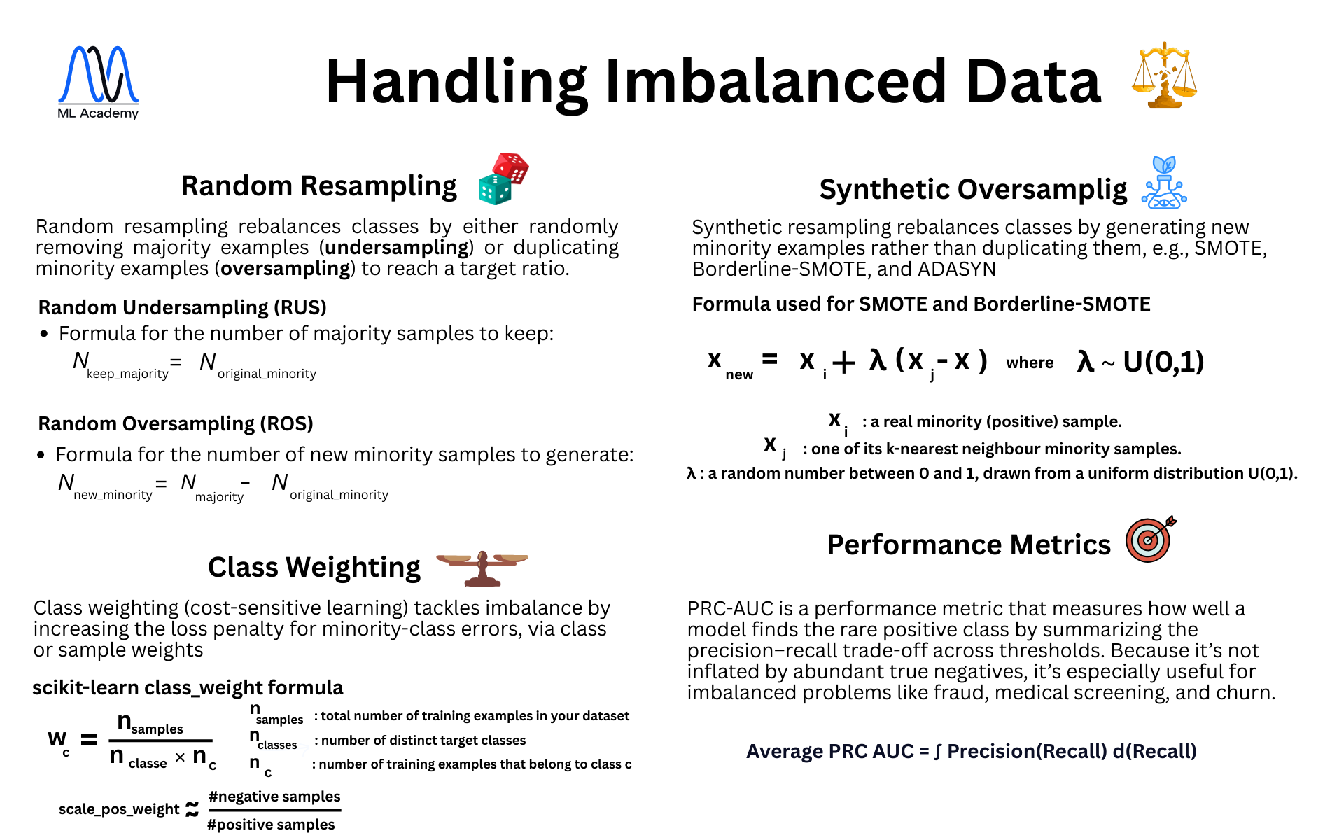
Balancing the Data: Undersampling, Oversampling, and Synthetic Sampling (SMOTE, Borderline-SMOTE, ADASYN)

When one class dominates, the model may learn to ignore the minority class. To address this, we can rebalance the dataset before training.

There are many methods for handling imbalanced data, and the most common are:

• Undersampling
• Oversampling
• SMOTE
• Borderline-SMOTE
• ADASYN

There are other approaches, but these are the most widely used. All of them aim to bring the proportions of the positive and negative classes closer together to create a more balanced dataset, either by removing samples from the majority class (Undersampling) or by increasing the number of samples in the minority class (Oversampling, SMOTE, SMOTE-Borderline, or ADASYN), which we will cover below.

Random Undersampling

Random undersampling is a technique used to balance class distributions in imbalanced datasets by randomly reducing the number of samples in the majority class. This approach helps to speed up training and can reduce model overfitting by limiting the dominance of the majority class. However, it carries the risk of discarding valuable information, which can affect model performance if important majority patterns are lost.

import pandas as pd
from imblearn.under_sampling import RandomUnderSampler # pip install imbalanced-learn


# 1) Load data
path = "/YourPath/fraud_data.csv"
df = pd.read_csv(path)


# 2) Basic cleaning
df = df.drop_duplicates()
# Drop high-cardinality / PII-like string columns that aren't useful for modeling
df = df.drop(columns=["nameDest", "nameOrig"])


# 3) Encode categorical 'type' into 0/1 columns so models can use it
df = pd.get_dummies(df, columns=["type"], dtype="uint8")


# 4) Separate target (label) and features + train / test split
#instead of using the train_test_split I will split my data based on the chronological step
df_train = df[df["step"]<=400]
df_test = df[df["step"]>400]
# X, y
X_train = df_train.drop(columns=["isFraud", "isFlaggedFraud"])
y_train = df_train["isFraud"]


X_test = df_test.drop(columns=["isFraud", "isFlaggedFraud"])
y_test = df_test["isFraud"]

# 5) Fix class imbalance on the TRAIN SET ONLY using SMOTE
rus = RandomUnderSampler(random_state=42)
X_under, y_under = rus.fit_resample(X_train, y_train)


# 6) Show class balance before/after
print("RandomOverSampler")
# This prints the percentage of the negative class (0) and the positive class (1) before SMOTE
print(" before:", pd.Series(y_train).value_counts(normalize=True).sort_index().to_dict())
# This prints the percentage of the negative class (0) and the positive class (1) after SMOTE
print(" after :", pd.Series(y_under).value_counts(normalize=True).sort_index().to_dict())

Results:

RandomOverSampler

before: {0: 0.9992263734592701, 1: 0.0007736265407298736}

after : {0: 0.5, 1: 0.5}

We see that the original training data are severely imbalanced (positives ≈ 0.13%). 

Random undersampling reduces the majority-class samples to balance class frequencies to (0.5, 0.5 instead of 0.99, 0.001), preventing the model from being dominated by negatives and often speeding up training. This is applied only during training, while the test set retains its true proportions to ensure unbiased evaluation. The trade-off: some majority-class information is lost.

Random Undersampling Pros:

Undersampling is an effective approach to address class imbalance by reducing the majority class size. The following advantages highlight why it can be a smart choice in many scenarios:

• Reduces computational cost by shrinking the majority class, speeding up training and lowering memory usage.

• Balances class representation to prevent model bias toward the majority class and improve minority class detection.
• Enhances performance for imbalance-sensitive algorithms (e.g., logistic regression, SVM) by focusing learning on minority patterns.
• Maintains simplicity and data integrity, as random undersampling avoids synthetic data generation common in oversampling.
• Reduces noise through informed methods like Tomek Links and NearMiss, which remove redundant or borderline majority samples.
• Improves interpretability by clarifying minority class signals through reduced majority class complexity.

Random Undersampling Cons:

Undersampling can be a valuable technique for addressing class imbalance. However, it presents several risks and limitations that must be carefully managed to prevent negative impacts on model performance. Key considerations include:

• Causes information loss by discarding the majority samples, which may remove rare but important patterns, potentially reducing AUROC and overall accuracy.
• Introduces sampling bias, as the retained majority subset may not fully represent the true data distribution, increasing variance and reducing model stability.
• Risks underfitting the majority class, leading to poorer performance when accurate majority predictions are operationally important.
• Risks of removing key samples near class boundaries, weakening the model’s ability to distinguish closely related classes.
• Alters class proportions, causing predicted probabilities to shift and requiring recalibration or adjustment.
• Results can be sensitive to random seed and sampling strategy, requiring careful control to ensure reproducibility.
• Does not address intrinsic class overlap or data noise, so these issues remain unresolved.
• Is fragile with small datasets, where further reduction amplifies variance and hampers learning.
• Carries process risks: must be confined to training folds after data splitting to avoid leakage and overly optimistic evaluation.

‍Trade-off: While undersampling can improve minority class performance, it may reduce overall model generalization due to information loss from the majority class. Best used when you have an abundant majority class data.

Random Oversampling

Random Oversampling: duplicates examples from the minority class until the classes are roughly balanced. It’s simple and effective, but can lead to overfitting because the same minority samples appear multiple times.

Code:

import pandas as pd
from imblearn.over_sampling import RandomOverSampler # pip install imbalanced-learn


# 1) Load data
path = "/YourPath/fraud_data.csv"
df = pd.read_csv(path)


# 2) Basic cleaning
df = df.drop_duplicates()
# Drop high-cardinality / PII-like string columns that aren't useful for modeling
df = df.drop(columns=["nameDest", "nameOrig"])


# 3) Encode categorical 'type' into 0/1 columns so models can use it
df = pd.get_dummies(df, columns=["type"], dtype="uint8")


# 4) Separate target (label) and features + train / test split
#instead of using the train_test_split I will split my data based on the chronological step
df_train = df[df["step"]<=400]
df_test = df[df["step"]>400]
# X, y
X_train = df_train.drop(columns=["isFraud", "isFlaggedFraud"])
y_train = df_train["isFraud"]


X_test = df_test.drop(columns=["isFraud", "isFlaggedFraud"])
y_test = df_test["isFraud"]


# 5) Fix class imbalance on the TRAIN SET ONLY using SMOTE
ros = RandomOverSampler(random_state=42)
X_over, y_over = ros.fit_resample(X_train, y_train)


# 6) Show class balance before/after
print("RandomOverSampler")
# This prints the percentage of the negative class (0) and the positive class (1) before SMOTE
print(" before:", pd.Series(y_train).value_counts(normalize=True).sort_index().to_dict())
# This prints the percentage of the negative class (0) and the positive class (1) after SMOTE
print(" after :", pd.Series(y_over).value_counts(normalize=True).sort_index().to_dict())

Results:

RandomOverSampler

before: {0: 0.9992263734592701, 1: 0.0007736265407298736}

after : {0: 0.5, 1: 0.5}

The original training data are severely imbalanced (positives ≈ 0.13%). To address this, random oversampling is applied: it duplicates minority-class examples so the training set represents both classes equally, allowing the model to learn positive cases more effectively. Oversampling is limited to the training phase; test data retain their natural ratios to ensure realistic, unbiased evaluation.

Random Oversampling Pros:

Random oversampling addresses class imbalance by duplicating minority class samples to increase their representation. This technique enables the model to better learn minority class patterns without losing any majority class data. Below are the key advantages that make random oversampling a useful choice in many scenarios:

• Balances class representation by increasing minority class samples to reduce bias toward the majority class.
• Enhances minority class learning by duplicating examples, often improving recall and precision metrics.
• Maintains simplicity and data integrity, as it replicates existing samples without generating synthetic data.
• Offers flexible control over the minority-to-majority ratio, allowing tailored class balance.
• Preserves a stable feature space, which supports model interpretability and auditability.
• Integrates easily into training pipelines and cross-validation workflows without special handling.
• Serves as a reliable baseline method against which more complex oversampling techniques can be compared.
• Ensures reproducibility when using a fixed random seed, facilitating consistent experimental results.

Random Oversampling Cons:

Random oversampling is a popular technique for handling class imbalance by duplicating minority class examples. However, it introduces several risks and limitations that must be carefully managed to avoid adverse impacts on model performance. Key considerations include:

• Increases overfitting risk by encouraging memorization of duplicated minority samples.
• Adds no new information since duplicates simply repeat existing points without enriching decision boundaries.
• Amplifies noise and outliers by replicating mislabeled or anomalous minority samples, potentially harming model robustness.
• Extends training time and memory usage due to the expanded effective dataset size.
• Alters class proportions, causing predicted probability shifts that require post-hoc calibration.
• Biases algorithms sensitive to duplicates (e.g., k-NN), which can distort local feature space structure.
• Fails to resolve intrinsic class overlap, as duplication alone cannot improve class separability.
• Carries leakage risk if applied before train-test splits or outside cross-validation folds, contaminating evaluation.
• Can degrade overall accuracy by increasing false positives even as minority recall improves.

Synthetic Sampling

SMOTE (Synthetic Minority Oversampling Technique)

SMOTE (Synthetic Minority Oversampling Technique) addresses class imbalance by synthesizing new minority class examples instead of duplicating existing ones. For each minority point xi, it identifies its 

k-nearest minority neighbors and generates synthetic samples along the line segments connecting xi to its neighbors:                                      

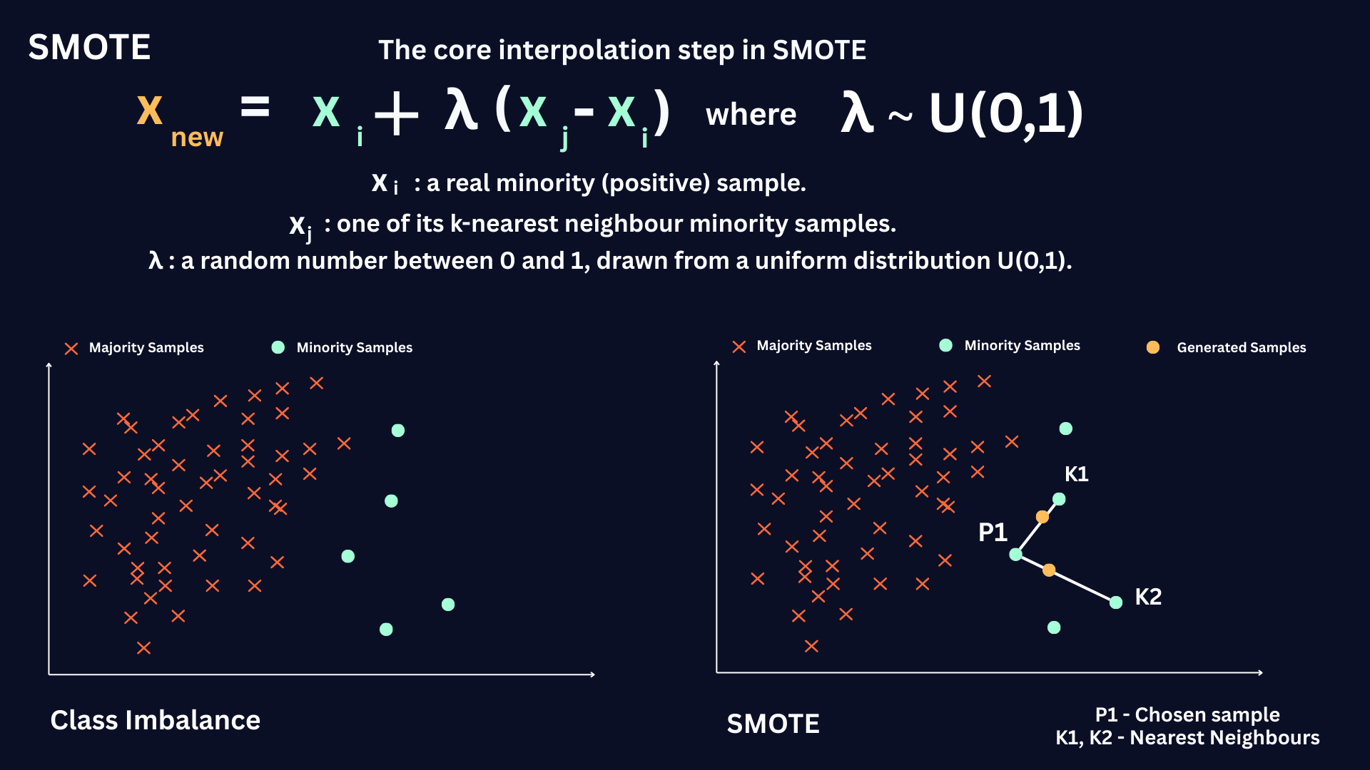
This approach expands the minority manifold in feature space, smoothing decision boundaries and typically improving recall and precision-recall AUC compared to naive duplication.

In essence, by interpolating within minority neighborhoods, SMOTE reduces bias toward the majority class and avoids overfitting to exact duplicates, providing a stronger learning signal for imbalance-sensitive models such as linear classifiers, SVMs, and tree ensembles.

However, it is important to apply SMOTE cautiously, as it may sometimes introduce noise, generate unrealistic synthetic samples, or increase computational complexity, especially in datasets with overlapping classes or outliers.

import pandas as pd
from imblearn.over_sampling import SMOTE # pip install imbalanced-learn


# 1) Load data
path = "/YourPath/fraud_data.csv"
df = pd.read_csv(path)


# 2) Basic cleaning
df = df.drop_duplicates()
# Drop high-cardinality / PII-like string columns that aren't useful for modeling
df = df.drop(columns=["nameDest", "nameOrig"])


# 3) Encode categorical 'type' into 0/1 columns so models can use it
df = pd.get_dummies(df, columns=["type"], dtype="uint8")


# 4) Separate target (label) and features + train / test split
#instead of using the train_test_split I will split my data based on the chronological step
df_train = df[df["step"]<=400]
df_test = df[df["step"]>400]
# X, y
X_train = df_train.drop(columns=["isFraud", "isFlaggedFraud"])
y_train = df_train["isFraud"]


X_test = df_test.drop(columns=["isFraud", "isFlaggedFraud"])
y_test = df_test["isFraud"]


# 5) Fix class imbalance on the TRAIN SET ONLY using SMOTE
sm = SMOTE(random_state=42, k_neighbors=5)
X_smote, y_smote = sm.fit_resample(X_train, y_train)


# 6) Show class balance before/after
print("SMOTE")
# This prints the percentage of the negative class (0) and the positive class (1) before SMOTE
print(" before:", pd.Series(y_train).value_counts(normalize=True).sort_index().to_dict())
# This prints the percentage of the negative class (0) and the positive class (1) after SMOTE
print(" after :", pd.Series(y_smote).value_counts(normalize=True).sort_index().to_dict())

Results:

SMOTE

before: {0: 0.9992263734592701, 1: 0.0007736265407298736}

after : {0: 0.5, 1: 0.5}

The original training data are severely imbalanced (positives ≈ 0.13%). SMOTE synthesizes new minority-class examples by interpolating between nearest neighbors, balancing class proportions to 0.5 each instead of the original extreme imbalance. This resampling is applied only during training; the test set preserves natural ratios for unbiased evaluation.

SMOTE Pros:

SMOTE offers an effective solution for class imbalance by creating new synthetic minority examples through interpolation. The following benefits illustrate why SMOTE can be a suitable choice in certain modeling contexts.

• Expands the minority class manifold by creating synthetic samples, improving decision boundary smoothness and minority class representation.
• Reduces bias toward the majority class by interpolating within minority neighborhoods, providing a stronger learning signal for imbalance-sensitive models.
• Maintains feature space continuity without introducing unrealistic outlier samples when properly tuned.
• Integrates well with cross-validation and pipeline workflows when applied correctly.

SMOTE Cons:

SMOTE can be a valuable technique for addressing class imbalance by synthesizing new minority samples. However, it presents several risks and limitations that must be carefully managed to prevent negative impacts on model performance. Key considerations include:

• Generates synthetic samples in minority regions that overlap with majority areas, potentially creating spurious "bridges" that increase class overlap and boundary noise.
• Propagates outliers because minority points deep in majority regions produce synthetic points that invade majority space ("class bridging"), amplifying noise.
• Does not account for majority class distribution when creating synthetic samples, which may reduce overall data representativeness.
• Can introduce noise if synthetic samples are created near mislabeled or ambiguous points.
• Increases computational complexity, especially with large datasets due to k-nearest neighbors calculations.
• Sensitive to the choice of k (number of neighbors), impacting the quality of synthetic samples.
• May reduce model calibration accuracy, skewing predicted probabilities.
• Less effective in high-dimensional feature spaces where interpolated samples may not capture complex patterns.
• Requires careful application to avoid data leakage and maintain valid validation protocols.

Note: The figures above use a different (synthetic) dataset than our earlier example. This is intentional: the data was designed to make SMOTE’s potential “bridging” behavior visible, synthetic points can be generated across regions dominated by the majority class, increasing overlap.

The figure shows SMOTE’s synthetic samples (highlighted) and how they can unintentionally connect minority and majority regions. This “bridging” increases overlap near the boundary and may confuse the classifier, especially when minority points lie close to or inside majority space.

SMOTE synthesizes new minority instances without explicitly accounting for the geometry of the majority class, which can increase class overlap in feature space. In the figure above, we project the imbalanced dataset before and after applying SMOTE; the post-SMOTE plot shows substantially more mixing between minority and majority points, illustrating how synthetic samples can “bridge” the two classes.

When minority instances are embedded deep within majority regions, SMOTE can generate synthetic samples that form artificial bridges across class boundaries, propagating outliers and intensifying class overlap. This happens because SMOTE interpolates along line segments connecting each minority point to its k nearest minority neighbors. If a minority outlier lies inside the majority manifold, the resulting synthetic points may extend through majority space, creating class bridging and amplifying boundary noise.

Class bridging:

Class bridging occurs when oversampling methods like SMOTE generate synthetic minority samples that spill into majority regions, forming artificial connections between classes. These synthetic bridges expand the minority boundary into majority space, introduce additional overlap and boundary noise, and often confuse the classifier.

Borderline-SMOTE

Borderline-SMOTE is a smarter variation of SMOTE that focuses on the regions where the classifier struggles most, the decision boundary. Instead of generating synthetic samples everywhere in the minority class, it zooms in on minority points surrounded by many majority neighbors. These are the “danger” points, which lie right where misclassifications usually happen.

The algorithm starts by running a KNN search to examine each minority sample’s neighborhood. It then labels each point as:

• Noise, if all neighbors are majority (likely outliers).

• Safe, if most neighbors are minority (already well represented).

• Danger, if majority neighbors dominate (close to the decision boundary).

Synthetic minority samples are created only from these danger points by interpolating with their minority neighbors. This targeted oversampling sharpens the boundary between classes, reduces noise from irrelevant regions, and helps the model focus its learning power where it matters most. Like any oversampling technique, it can still be sensitive to noisy edges and requires careful tuning, but it often delivers more stable and realistic gains than standard SMOTE.

Borderline-SMOTE generates synthetic samples only from minority “danger” points, instances near the class boundary with many majority neighbours, to reinforce the decision boundary where errors are most likely.

import pandas as pd
from imblearn.over_sampling import BorderlineSMOTE # pip install imbalanced-learn


# 1) Load data
path = "/YourPath/fraud_data.csv"
df = pd.read_csv(path)


# 2) Basic cleaning
df = df.drop_duplicates()
# Drop high-cardinality / PII-like string columns that aren't useful for modeling
df = df.drop(columns=["nameDest", "nameOrig"])


# 3) Encode categorical 'type' into 0/1 columns so models can use it
df = pd.get_dummies(df, columns=["type"], dtype="uint8")


# 4) Separate target (label) and features + train / test split
#instead of using the train_test_split I will split my data based on the chronological step
df_train = df[df["step"]<=400]
df_test = df[df["step"]>400]
# X, y
X_train = df_train.drop(columns=["isFraud", "isFlaggedFraud"])
y_train = df_train["isFraud"]


X_test = df_test.drop(columns=["isFraud", "isFlaggedFraud"])
y_test = df_test["isFraud"]


# 5) Fix class imbalance on the TRAIN SET ONLY using Borderline-SMOTE
sm = BorderlineSMOTE(
   random_state=42,
   k_neighbors=5,
   kind="borderline-1"   # or "borderline-2"
)
X_smote, y_smote = sm.fit_resample(X_train, y_train)


# 6) Show class balance before/after
print("SMOTE")
# This prints the percentage of the negative class (0) and the positive class (1) before SMOTE
print(" before:"                                                          , pd.Series(y_train).value_counts(normalize=True).sort_index().to_dict())
# This prints the percentage of the negative class (0) and the positive class (1) after SMOTE
print(" after :"                                                          , pd.Series(y_smote).value_counts(normalize=True).sort_index().to_dict())

Results:

Borderline-SMOTE

before: {0: 0.9992263734592701, 1: 0.0007736265407298736}

after : {0: 0.5, 1: 0.5}

Borderline-SMOTE Pros

Borderline-SMOTE refines standard SMOTE by focusing oversampling on “danger” minority points, those near majority neighbours, so the model learns a sharper and more informative decision boundary.

• Targets high-risk regions near the decision boundary, where misclassifications are most likely, instead of oversampling everywhere.
• Ignores noise points (minority samples surrounded only by majority), reducing the risk of propagating clear outliers compared to vanilla SMOTE.
• Generates synthetic samples around informative borderline examples, often improving recall on the minority class in difficult, overlapping regions.
• Can produce a cleaner, more discriminative boundary by reinforcing minority presence where the classes interact most.
• Often works better than basic SMOTE when the problem is “hard boundary” rather than purely sparse minority regions.

Borderline-SMOTE Cons

Despite being more targeted than SMOTE, Borderline-SMOTE still brings important risks that must be managed carefully.

• If the boundary region itself is noisy or mislabeled, it will amplify that noise by generating more samples exactly there.
• Can overemphasize borderline areas and underrepresent safe minority regions, potentially distorting the true class distribution.
• Remains sensitive to k-NN choices (k and distance metric), which affects how “danger”, “safe”, and “noise” are defined.
• May still increase class overlap if danger points sit inside heavily mixed regions, leading to a fuzzier decision boundary.
• Adds extra computational and implementation complexity over standard SMOTE (two KNN passes + selective oversampling).
• Less suitable when the minority class is extremely sparse, since there may be too few meaningful neighbours to synthesize realistic samples.

Trade-off in practice

Borderline-SMOTE is a more surgical alternative to SMOTE: it usually reduces the propagation of clear outliers and strengthens the classifier exactly where errors cluster (the boundary). However, that same focus on borderline regions can backfire when the boundary is noisy or poorly understood. It’s often a good choice when you have moderate overlap and a reasonably clean boundary, but it still requires careful tuning (k, oversampling rate) and robust validation to avoid overfitting or boundary noise.

ADASYN

Building further, ADASYN (Adaptive Synthetic Sampling) adapts synthetic sample generation based on local learning difficulty. It creates more synthetic points in regions where the minority class is hardest to learn and fewer where classification is easier. This dynamic approach tends to improve recall on complex or scattered minority distributions. However, it requires cautious tuning to avoid overemphasizing noise or mislabeled data, often necessitating conservative sampling parameters and subsequent cleaning.

import pandas as pd
from imblearn.over_sampling import ADASYN # pip install imbalanced-learn


# 1) Load data
path = "/YourPath/fraud_data.csv"
df = pd.read_csv(path)


# 2) Basic cleaning
df = df.drop_duplicates()
# Drop high-cardinality / PII-like string columns that aren't useful for modeling
df = df.drop(columns=["nameDest", "nameOrig"])


# 3) Encode categorical 'type' into 0/1 columns so models can use it
df = pd.get_dummies(df, columns=["type"], dtype="uint8")


# 4) Separate target (label) and features + train / test split
#instead of using the train_test_split I will split my data based on the chronological step
df_train = df[df["step"]<=400]
df_test = df[df["step"]>400]
# X, y
X_train = df_train.drop(columns=["isFraud", "isFlaggedFraud"])
y_train = df_train["isFraud"]


X_test = df_test.drop(columns=["isFraud", "isFlaggedFraud"])
y_test = df_test["isFraud"]


# 5) Fix class imbalance on the TRAIN SET ONLY using ADASYN
adasyn = ADASYN(
   random_state=42,
   n_neighbors=5,          # similar role to k_neighbors in SMOTE/Borderline-SMOTE
   sampling_strategy="auto"
)
X_res, y_res = adasyn.fit_resample(X_train, y_train)


# 6) Show class balance before/after
print("ADASYN") 
# This prints the percentage of the negative class (0) and the positive class (1) before SMOTE
print(" before:", pd.Series(y_train).value_counts(normalize=True).sort_index().to_dict())
# This prints the percentage of the negative class (0) and the positive class (1) after SMOTE
print(" after :", pd.Series(y_res).value_counts(normalize=True).sort_index().to_dict())

Results:

ADASYN

before: {0: 0.9992263734592701, 1: 0.0007736265407298736}

after : {0: 0.4999999135330167, 1: 0.5000000864669832}

ADASYN Pros

ADASYN (Adaptive Synthetic Sampling) is a variant of SMOTE that can improve performance in certain scenarios. Here are some of its main advantages:

• Focuses on oversampling hard-to-learn minority points surrounded by majority neighbors, extending SMOTE’s idea with adaptive weighting.
• Automatically emphasizes regions where the minority class is hardest to classify, generating more synthetic samples there.
• Improves minority recall more effectively than uniform SMOTE by targeting difficult regions rather than oversampling evenly.
• Adapts dynamically to local class imbalance, producing a richer distribution of synthetic samples along complex boundaries.
• Reduces manual tuning, its weighting mechanism automatically redistributes synthetic samples based on per-point difficulty.
• Integrates smoothly into modeling pipelines and cross-validation when applied correctly (inside the CV loop).
• Works best in datasets with uneven minority difficulty, where some clusters are well represented and others sparse.

ADASYN Cons

While ADASYN often outperforms basic oversampling methods, it is not risk-free; several things can go wrong if it’s applied without care:

• By focusing on hard regions, it can amplify noise or ambiguity if those areas contain mislabeled or overlapping samples.
• May worsen boundary confusion if the algorithm generates many synthetic points in noisy regions.
• Sensitive to parameter choices (k in k-NN, sampling ratios, and desired imbalance), which strongly influence outcomes.
• Can distort the distribution by overpopulating ambiguous regions while undersampling safer ones.
• Inherits SMOTE’s computational and distance-metric sensitivities, especially in high-dimensional data.
• May reduce model calibration quality due to aggressive oversampling near uncertain boundaries.
• Performs poorly when the minority class is extremely sparse or noisy, as adaptive weights overemphasize unreliable points.

Trade-off in Practice

ADASYN is a more adaptive and assertive cousin of SMOTE. It often boosts minority recall by generating samples in challenging regions, outperforming uniform SMOTE when local difficulty drives imbalance. But that same adaptivity can be a liability if “hard” means noisy or mislabeled, ADASYN will amplify those flaws. It works best when data are pre-cleaned, applied inside cross-validation, and evaluated with precision, recall, and calibration in mind to ensure the performance gains reflect genuine learning rather than noise amplification.

SMOTE Methods Summary

While SMOTE treats all minority samples equally, its adaptive variant ADASYN shifts focus toward the harder-to-classify examples, often located in sparse or overlapping regions. By estimating the local classification difficulty of each minority instance, ADASYN builds a weighted sampling distribution that prioritizes generating new data exactly where the model struggles most.

In practice, random oversampling and undersampling still provide simple baselines but risk redundancy or information loss. Modern geometry-aware techniques like SMOTE, Borderline-SMOTE, and ADASYN refine this process by shaping the synthetic data generation around the topology of the decision boundary. When applied thoughtfully, within cross-validation, with parameter tuning and noise control, these methods help models learn more balanced, discriminative, and generalizable decision surfaces.

Strategies that can be followed for better results

Strategies to follow for Better Results with Oversampling:

Combine SMOTE with undersampling

First apply SMOTE to increase the number of minority samples, then perform random undersampling (or use a more sophisticated undersampler) on the majority class. This helps balance the dataset without excessively increasing its size and reduces majority dominance in overlapping regions.

Remove outliers and reduce noise before using ADASYN

Clean the data (e.g., by dropping clear minority outliers or suspected mislabeled samples) before applying ADASYN. Because ADASYN focuses on “hard” regions, removing noisy or unreliable points prevents it from generating many synthetic samples around bad data.

Tune k and the sampling ratio conservatively

Use smaller values of k (fewer neighbors) and moderate oversampling ratios to avoid creating too many synthetic samples in heavily mixed regions. Start with mild oversampling (e.g., 20–50%) and increase only when performance metrics justify it.

Apply SMOTE/ADASYN inside cross-validation folds

Always oversample after splitting and within each cross-validation fold to avoid data leakage. This ensures that validation sets remain representative of real-world imbalance and prevents overly optimistic performance estimates.

Scale and encode features appropriately before oversampling

Standardize or normalize continuous features and use a suitable encoding (or SMOTE-NC) for categorical variables. Distance-based methods like SMOTE and ADASYN rely on meaningful distance calculations, which in turn depend on proper feature scaling and encoding.

Monitor precision, PR-AUC, and calibration - not just recall

After oversampling, evaluate false positives, precision, PR-AUC, and probability calibration in addition to recall. This helps identify situations where oversampling improves minority recall but degrades overall reliability or makes predictions too noisy for practical use.

When dealing with Imbalanced data, always keep in mind the flow below

When dealing with imbalanced data, it is useful to start from the simplest resampling approaches and understand their trade-offs. Random oversampling increases the minority class by duplicating rare examples. This quickly raises the number of positives in the training set and can improve recall, but it also encourages the model to memorize those duplicates rather than learn a robust decision boundary, inflating training metrics without necessarily improving generalization. Random undersampling, in contrast, reduces the majority class.

This can sharpen the classifier and shorten training time, but it discards a substantial amount of useful majority-class information, increases variance, and can harm probability calibration. In short, oversampling tends to overfit, while undersampling risks throwing away important signals.

SMOTE is often introduced as a more sophisticated alternative. Instead of copying minority samples, it interpolates between neighbouring minority points to synthesize new examples. This can better populate the minority manifold, smooth the decision boundary, and enhance recall.

However, because SMOTE does not explicitly model the majority-class geometry, synthetic samples can “bridge” across class boundaries, especially around outliers or in highly mixed regions, leading to increased overlap between classes and a reduction in precision. These issues are amplified in high-dimensional feature spaces, where nearest-neighbour relationships are less reliable. Moreover, if SMOTE is applied before a proper train/validation split, it introduces leakage and produces overly optimistic evaluation results.

When You Don’t Want to Touch the Data

Sometimes, resampling isn’t an option, especially when working with sensitive or production datasets. In these cases, we can still handle imbalance by focusing on model evaluation, threshold tuning, and class weighting rather than changing the data itself.

Many modern algorithms let you change how much each class contributes to the loss. Instead of duplicating minority samples, you tell the model: “errors on this class are more expensive.”

In scikit-learn models such as Logistic Regression and Random Forest, setting class_weight="balanced" automatically computes a weight for each class c:

Because n𝑐 appears in the denominator, rare classes (small n𝑐 ) get larger weights w𝑐, and very common classes (large n𝑐 ) get smaller weights. Misclassifying a minority example therefore “hurts” the loss more than misclassifying a majority example, nudging the model to pay more attention to under-represented cases without any resampling.

XGBoost uses the same idea via the scale_pos_weight parameter in binary classification. This parameter multiplies the loss (gradient and Hessian) for positive examples only. A common rule of thumb is:

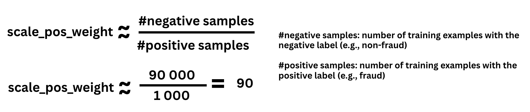
This means an error on a fraud sample counts roughly 90× more than an error on a non-fraud sample in the XGBoost loss. In practice, this pushes the model to stop “playing it safe” by predicting the majority class everywhere, even though the underlying data distribution is unchanged.

The key is to use metrics that truly reflect performance on the minority class. Instead of relying on accuracy, look at:

• Precision: how many of the predicted positives are correct
• Recall: how many of the actual positives were found
• F1-score: a balance between the two (often more informative per class than a single global F1)

You can visualize these trade-offs using the Precision–Recall Curve (PRC), which shows how precision and recall change as you move the decision threshold. This helps you choose an operating point that matches the business cost of false positives vs. false negatives, especially in highly imbalanced settings.

The Average PRC-AUC - a go-to metric for imbalanced data

Among all evaluation metrics for imbalanced datasets, none captures reality better than the Average Precision–Recall Curve AUC (Average PRC–AUC).

While ROC-AUC is widely used, it can be misleading on skewed data because it includes the True Negative (TN) rate in its calculation, and when the negative class dominates, this can inflate the score and make a weak model look good.

In contrast, PRC-AUC focuses only on the positive (minority) class, evaluating how well the model identifies those rare but critical cases. It completely ignores TNs, which prevents bias toward the majority class and makes it far more meaningful for problems like fraud detection, medical diagnosis, and churn prediction.

Mathematically:

A high Average PRC-AUC means your model achieves strong recall without sacrificing too much precision,  it finds what matters most while staying accurate.

Rule of thumb:

When classes are highly imbalanced, always prefer PRC-AUC over ROC-AUC, it tells the real story of your model’s performance.

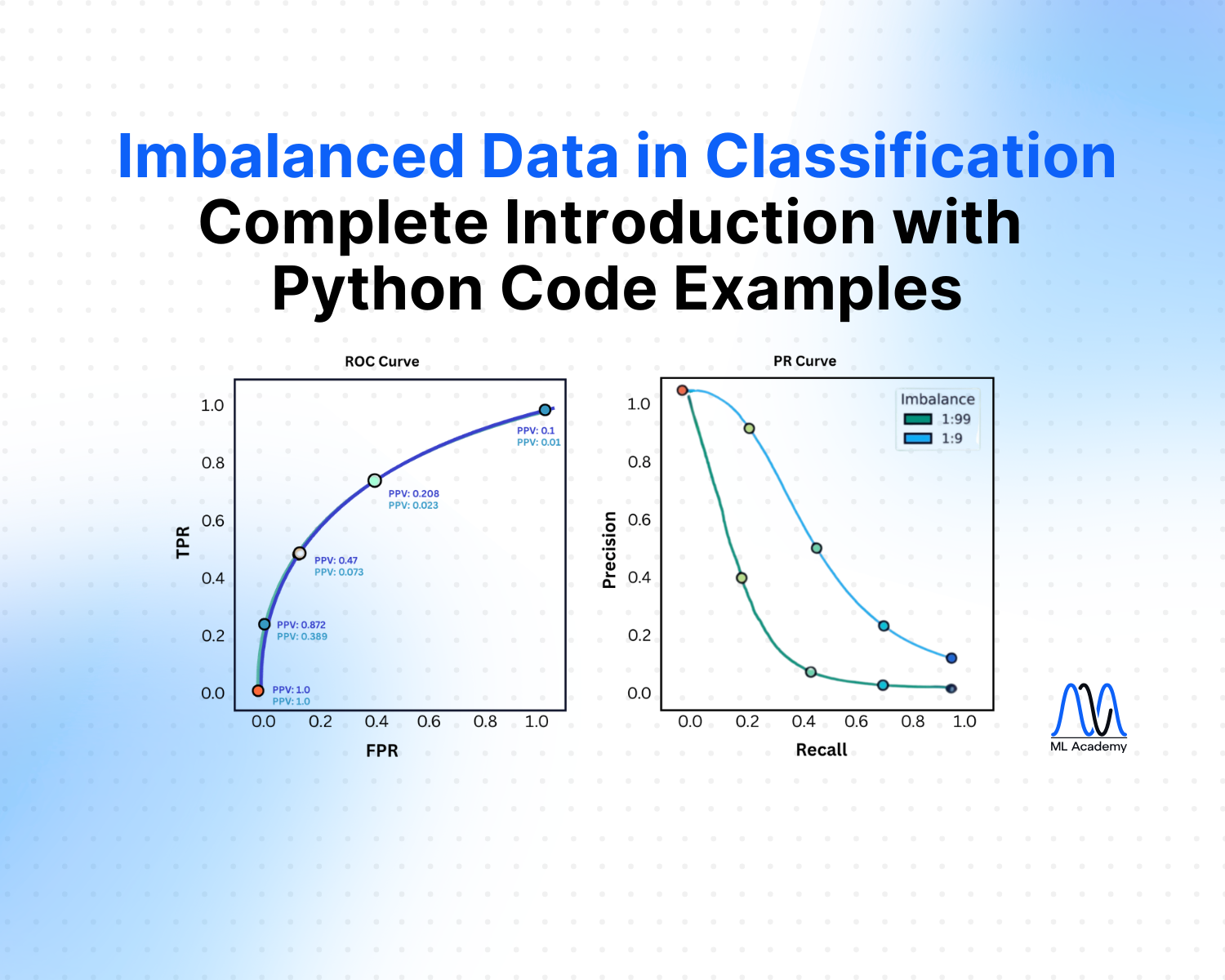
This figure compares ROC and PR curves under two different class-imbalance ratios (1:9 in blue, 1:99 in green). 

On the left, the ROC curve looks almost identical for both settings: even when positives become much rarer, the TPR–FPR trade-off barely changes and ROC-AUC stays high, which can give a false sense of model quality. 

On the right, the PR curves tell a different story: as imbalance increases to 1:99, precision drops sharply across all recall levels, revealing that most predicted positives are actually false alarms. 

Together, the plots highlight that ROC-AUC is relatively insensitive to class imbalance, while PR-AUC and the precision–recall curve more accurately reflect performance on rare-event detection problems such as fraud.

In the next section, we’ll examine how resampling methods impact model performance and see how the pros and cons of each method show up in the results.

Key Takeaways

• Don’t trust accuracy on its own. In heavily imbalanced settings, prioritize per-class Precision, Recall, F1-score, and PRC-AUC. Use Accuracy, Specificity, and FPR/FNR mainly as guardrail metrics rather than primary objectives.

• Use SMOTE and its variants with care. SMOTE interpolates between minority neighbours to create synthetic samples and often outperforms plain random oversampling, but it can “bridge” into majority regions (especially when minority outliers sit inside majority space) and increase class overlap. Borderline-SMOTE and ADASYN can mitigate some of this, but they inherit similar risks and require tuning.

• Never resample before splitting. Always apply any resampling method (undersampling, oversampling, SMOTE, Borderline-SMOTE, ADASYN) after the train–test split and inside cross-validation folds to avoid leakage and overly optimistic metrics.

• Average PRC-AUC should be the default metric for rare events. It focuses purely on the minority class and ignores true negatives, making it far more informative than ROC-AUC when positives are rare.

• Choose between resampling and class weighting based on constraints. If you can safely modify the data, resampling can improve minority recall; if not (e.g., production, governance, or storage constraints), rely on class-weighted models, threshold tuning, and careful evaluation instead.

• Tune thresholds using the precision–recall curve. Use the PR curve to understand the trade-off between catching more positives (recall) and limiting false alarms (precision), then pick operating points that align with business costs and risk tolerance.